Introduction
One of the most common questions we get on Analytics Vidhya is,
How much maths do I need to learn to be a data scientist?
Even though the question sounds simple, there is no simple answer to the the question. Usually, we say that you need to know basic descriptive and inferential statistics to start. That is good to start.
But, once you have covered the basic concepts in machine learning, you will need to learn some more math. You need it to understand how these algorithms work. What are their limitations and in case they make any underlying assumptions. Now, there could be a lot of areas to study including algebra, calculus, statistics, 3-D geometry etc.
If you get confused (like I did) and ask experts what should you learn at this stage, most of them would suggest / agree that you go ahead with Linear Algebra.
But, the problem does not stop there. The next challenge is to figure out how to learn Linear Algebra. You can get lost in the detailed mathematics and derivation and learning them would not help as much! I went through that journey myself and hence decided to write this comprehensive guide.
If you have faced this question about how to learn & what to learn in Linear Algebra – you are at the right place. Just follow this guide.
And if you’re looking to understand where linear algebra fits into the overall data science scheme, here’s the perfect article:
Table of contents
- Motivation – Why learn Linear Algebra?
- Representation of problems in Linear Algebra
2.1. Visualising the problem: Line
2.2. Complicate the problem
2.3. Planes - Matrix
3.1 Terms related to Matrix
3.2 Basic operations on Matrix
3.3 Representing in Matrix form - Solving the problem
4.1. Row Echelon form
4.2. Inverse of a Matrix
4.2.1 Finding Inverse
4.2.2 The power of Matrices: solving the equations in one go
4.2.3 Use of Inverse in Data Science - Eigenvalues and Eigenvectors
5.1 Finding Eigenvectors
5.2 Use of Eigenvectors in Data Science: PCA algorithm - Singular Value Decomposition of a Matrix
- End Notes
1. Motivation – Why learn Linear Algebra?
I would like to present 4 scenarios to showcase why learning Linear Algebra is important, if you are learning Data Science and Machine Learning.
Scenario 1:
![]()
What do you see when you look at the image above? You most likely said flower, leaves -not too difficult. But, if I ask you to write that logic so that a computer can do the same for you – it will be a very difficult task (to say the least).
You were able to identify the flower because the human brain has gone through million years of evolution. We do not understand what goes in the background to be able to tell whether the colour in the picture is red or black. We have somehow trained our brains to automatically perform this task.
But making a computer do the same task is not an easy task, and is an active area of research in Machine Learning and Computer Science in general. But before we work on identifying attributes in an image, let us ponder over a particular question- How does a machine stores this image?
You probably know that computers of today are designed to process only 0 and 1. So how can an image such as above with multiple attributes like colour be stored in a computer? This is achieved by storing the pixel intensities in a construct called Matrix. Then, this matrix can be processed to identify colours etc.
So any operation which you want to perform on this image would likely use Linear Algebra and matrices at the back end.
Scenario 2:
If you are somewhat familiar with the Data Science domain, you might have heard about the world “XGBOOST” – an algorithm employed most frequently by winners of Data Science Competitions. It stores the numeric data in the form of Matrix to give predictions. It enables XGBOOST to process data faster and provide more accurate results. Moreover, not just XGBOOST but various other algorithms use Matrices to store and process data.
Scenario 3:
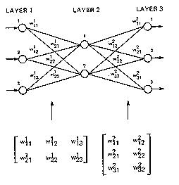
Deep Learning- the new buzz word in town employs Matrices to store inputs such as image or speech or text to give a state-of-the-art solution to these problems. Weights learned by a Neural Network are also stored in Matrices. Below is a graphical representation of weights stored in a Matrix.
Scenario 4:
Another active area of research in Machine Learning is dealing with text and the most common techniques employed are Bag of Words, Term Document Matrix etc. All these techniques in a very similar manner store counts(or something similar) of words in documents and store this frequency count in a Matrix form to perform tasks like Semantic analysis, Language translation, Language generation etc.
So, now you would understand the importance of Linear Algebra in machine learning. We have seen image, text or any data, in general, employing matrices to store and process data. This should be motivation enough to go through the material below to get you started on Linear Algebra. This is a relatively long guide, but it builds Linear Algebra from the ground up.
2. Representation of problems in Linear Algebra
Let’s start with a simple problem. Suppose that price of 1 ball & 2 bat or 2 ball and 1 bat is 100 units. We need to find price of a ball and a bat.
Suppose the price of a bat is Rs ‘x’ and the price of a ball is Rs ‘y’. Values of ‘x’ and ‘y’ can be anything depending on the situation i.e. ‘x’ and ‘y’ are variables.
Let’s translate this in mathematical form –
2x + y = 100 ...........(1)
Similarly, for the second condition-
x + 2y = 100 ..............(2)
Now, to find the prices of bat and ball, we need the values of ‘x’ and ‘y’ such that it satisfies both the equations. The basic problem of linear algebra is to find these values of ‘x’ and ‘y’ i.e. the solution of a set of linear equations.
Broadly speaking, in linear algebra data is represented in the form of linear equations. These linear equations are in turn represented in the form of matrices and vectors.
The number of variables as well as the number of equations may vary depending upon the condition, but the representation is in form of matrices and vectors.
2.1 Visualise the problem
It is usually helpful to visualize data problems. Let us see if that helps in this case.
Linear equations represent flat objects. We will start with the simplest one to understand i.e. line. A line corresponding to an equation is the set of all the points which satisfy the given equation. For example,
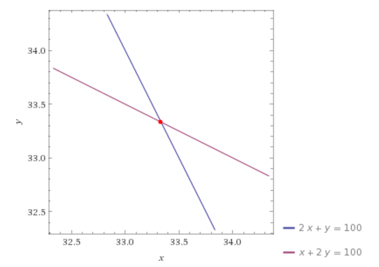
Points (50,0) , (0,100), (100/3,100/3) and (30,40) satisfy our equation (1) . So these points should lie on the line corresponding to our equation (1). Similarly, (0,50),(100,0),(100/3,100/3) are some of the points that satisfy equation (2).
Now in this situation, we want both of the conditions to be satisfied i.e. the point which lies on both the lines. Intuitively, we want to find the intersection point of both the lines as shown in the figure below.
Let’s solve the problem by elementary algebraic operations like addition, subtraction and substitution.
2x + y = 100 .............(1)
x + 2y = 100 ..........(2)
from equation (1)-
y = (100- x)/2
put value of y in equation (2)-
x + 2*(100-x)/2 = 100......(3)
Now, since the equation (3) is an equation in single variable x, it can be solved for x and subsequently y.
That looks simple – let’s go one step further and explore.
2.2 Let’s complicate the problem
Now, suppose you are given a set of three conditions with three variables each as given below and asked to find the values of all the variables. Let’s solve the problem and see what happens.
x+y+z=1.......(4)
2x+y=1......(5)
5x+3y+2z=4.......(6)
From equation (4) we get,
z=1-x-y....(7)
Substituting value of z in equation (6), we get –
5x+3y+2(1-x-y)=4
3x+y=2.....(8)
Now, we can solve equations (8) and (5) as a case of two variables to find the values of ‘x’ and ‘y’ in the problem of bat and ball above. Once we know‘x’ and ‘y’, we can use (7) to find the value of ‘z’.
As you might see, adding an extra variable has tremendously increased our efforts for finding the solution of the problem. Now imagine having 10 variables and 10 equations. Solving 10 equations simultaneously can prove to be tedious and time consuming. Now dive into data science. We have millions of data points. How do you solve those problems?
We have millions of data points in a real data set. It is going to be a nightmare to reach to solutions using the approach mentioned above. And imagine if we have to do it again and again and again. It’s going to take ages before we can solve this problem. And now if I tell you that it’s just one part of the battle, what would you think? So, what should we do? Should we quit and let it go? Definitely NO. Then?
Matrix is used to solve a large set of linear equations. But before we go further and take a look at matrices, let’s visualise the physical meaning of our problem. Give a little bit of thought to the next topic. It directly relates to the usage of Matrices.
2.3 Planes
A linear equation in 3 variables represents the set of all points whose coordinates satisfy the equations. Can you figure out the physical object represented by such an equation? Try to think of 2 variables at a time in any equation and then add the third one. You should figure out that it represents a three-dimensional analogue of line.
Basically, a linear equation in three variables represents a plane. More technically, a plane is a flat geometric object which extends up to infinity.
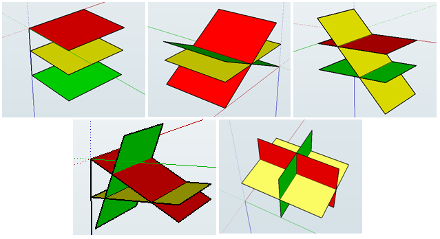
As in the case of a line, finding solutions to 3 variables linear equation means we want to find the intersection of those planes. Now can you imagine, in how many ways a set of three planes can intersect? Let me help you out. There are 4 possible cases –
- No intersection at all.
- Planes intersect in a line.
- They can intersect in a plane.
- All the three planes intersect at a point.
Can you imagine the number of solutions in each case? Try doing this. Here is an aid picked from Wikipedia to help you visualise.
So, what was the point of having you to visualise all graphs above?
Normal humans like us and most of the super mathematicians can only visualise things in 3-Dimensions, and having to visualise things in 4 (or 10000) dimensions is difficult impossible for mortals. So, how do mathematicians deal with higher dimensional data so efficiently? They have tricks up their sleeves and Matrices is one such trick employed by mathematicians to deal with higher dimensional data.
Now let’s proceed with our main focus i.e. Matrix.
3. Matrix
Matrix is a way of writing similar things together to handle and manipulate them as per our requirements easily. In Data Science, it is generally used to store information like weights in an Artificial Neural Network while training various algorithms. You will be able to understand my point by the end of this article.
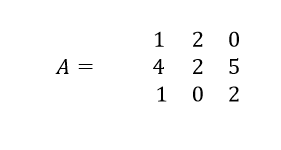
Technically, a matrix is a 2-D array of numbers (as far as Data Science is concerned). For example look at the matrix A below.
| 1 | 2 | 3 |
| 4 | 5 | 6 |
| 7 | 8 | 9 |
Generally, rows are denoted by ‘i’ and column are denoted by ‘j’. The elements are indexed by ‘i’th row and ‘j’th column.We denote the matrix by some alphabet e.g. A and its elements by A(ij).
In above matrix
A12 = 2
To reach to the result, go along first row and reach to second column.
3.1 Terms related to Matrix
Order of matrix – If a matrix has 3 rows and 4 columns, order of the matrix is 3*4 i.e. row*column.
Square matrix – The matrix in which the number of rows is equal to the number of columns.
Diagonal matrix – A matrix with all the non-diagonal elements equal to 0 is called a diagonal matrix.
Upper triangular matrix – Square matrix with all the elements below diagonal equal to 0.
Lower triangular matrix – Square matrix with all the elements above the diagonal equal to 0.
Scalar matrix – Square matrix with all the diagonal elements equal to some constant k.
Identity matrix – Square matrix with all the diagonal elements equal to 1 and all the non-diagonal elements equal to 0.
Column matrix – The matrix which consists of only 1 column. Sometimes, it is used to represent a vector.
Row matrix – A matrix consisting only of row.
Trace – It is the sum of all the diagonal elements of a square matrix.
3.2 Basic operations on matrix
Let’s play with matrices and realise the capabilities of matrix operations.
Addition – Addition of matrices is almost similar to basic arithmetic addition. All you need is the order of all the matrices being added should be same. This point will become obvious once you will do matrix addition by yourself.
Suppose we have 2 matrices ‘A’ and ‘B’ and the resultant matrix after the addition is ‘C’. Then
Cij = Aij + Bij
For example, let’s take two matrices and solve them.
A =
| 1 | 0 |
| 2 | 3 |
B =
| 4 | -1 |
| 0 | 5 |
Then,
C =
| 5 | -1 |
| 2 | 8 |
Observe that to get the elements of C matrix, I have added A and B element-wise i.e. 1 to 4, 3 to 5 and so on.
Scalar Multiplication – Multiplication of a matrix with a scalar constant is called scalar multiplication. All we have to do in a scalar multiplication is to multiply each element of the matrix with the given constant. Suppose we have a constant scalar ‘c’ and a matrix ‘A’. Then multiplying ‘c’ with ‘A’ gives-
c[Aij] = [c*Aij]
Transposition – Transposition simply means interchanging the row and column index. For example-
AijT= Aji
Transpose is used in vectorized implementation of linear and logistic regression.
Code in python
import numpy as np
#create a 3*3 matrix
A= np.arange(21,30).reshape(3,3)

#print the matrix
print('\n\nMatrix\n\n')
print(A)

print('\n\nTranspose of Matrix\n\n')
print(A.transpose())
Code in R
Output
[,1] [,2] [,3]
[1,] 11 12 13
[2,] 14 15 16
[3,] 17 18 19
t(A)
[,1] [,2] [,3]
[1,] 11 14 17
[2,] 12 15 18
[3,] 13 16 19
Matrix multiplication
Matrix multiplication is one of the most frequently used operations in linear algebra. We will learn to multiply two matrices as well as go through its important properties.
Before landing to algorithms, there are a few points to be kept in mind.
- The multiplication of two matrices of orders i*j and j*k results into a matrix of order i*k. Just keep the outer indices in order to get the indices of the final matrix.
- Two matrices will be compatible for multiplication only if the number of columns of the first matrix and the number of rows of the second one are same.
- The third point is that order of multiplication matters.
Don’t worry if you can’t get these points. You will be able to understand by the end of this section.
Suppose, we are given two matrices A and B to multiply. I will write the final expression first and then will explain the steps.
I have picked this image from Wikipedia for your better understanding.
In the first illustration, we know that the order of the resulting matrix should be 3*3. So first of all, create a matrix of order 3*3. To determine (AB)ij , multiply each element of ‘i’th row of A with ‘j’th column of B one at a time and add all the terms. To help you understand element-wise multiplication, take a look at the code below.
import numpy as np
A=np.arange(21,30).reshape(3,3)
B=np.arange(31,40).reshape(3,3)
A.dot(B)
So, how did we get 2250 as first element of AB matrix? 2250=21*31+22*34+23*37. Similarly, for other elements.
Code in R
A*B
[,1] [,2] [,3]
[1,] 220 252 286
[2,] 322 360 400
[3,] 442 486 532
Notice the difference between AB and BA.
Properties of matrix multiplication
- Matrix multiplication is associative provided the given matrices are compatible for multiplication i.e.
ABC = (AB)C = A(BC)
import numpy as np
A=np.arange(21,30).reshape(3,3)
B=np.arange(31,40).reshape(3,3)
C=np.arange(41,50).reshape(3,3)
temp1=(A.dot(B)).dot(C)
temp2=A.dot((B.dot(C)))
2. Matrix multiplication is not commutative i.e. AB and BA are not equal. We have verified this result above.
Matrix multiplication is used in linear and logistic regression when we calculate the value of output variable by parameterized vector method. As we have learned the basics of matrices, it’s time to apply them.
3.3 Representing equations in matrix form
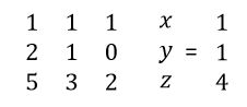
Let me do something exciting for you. Take help of pen and paper and try to find the value of the matrix multiplication shown below
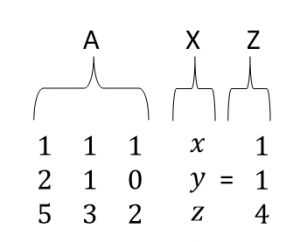
It can be verified very easily that the expression contains our three equations. We will name our matrices as ‘A’, ‘X’ and ‘Z’.
It explicitly verifies that we can write our equations together in one place as
AX = Z
Next step has to be solution methods.We will go through two methods to find the solution.
4. Solving the Problem
Now, we will look in detail the two methods to solve matrix equations.
- Row Echelon Form
- Inverse of a Matrix
4.1 Row Echelon form
Now you have visualised what an equation in 3 variables represents and had a warm up on matrix operations. Let’s find the solution of the set of equations given to us to understand our first method of interest and explore it later in detail.
I have already illustrated that solving the equations by substitution method can prove to be tedious and time taking. Our first method introduces you with a neater and more systematic method to accomplish the job in which, we manipulate our original equations systematically to find the solution. But what are those valid manipulations? Are there any qualifying criteria they have to fulfil? Well, yes. There are two conditions which have to be fulfilled by any manipulation to be valid.
- Manipulation should preserve the solution i.e. solution should not be altered on imposing the manipulation.
- Manipulation should be reversible.
So, what are those manipulations?
- We can swap the order of equations.
- We can multiply both sides of equations by any non-zero constant ‘c’.
- We can multiply an equation by any non-zero constant and then add to other equation.
These points will become more clear once you go through the algorithm and practice it. The basic idea is to clear variables in successive equations and form an upper triangular matrix. Equipped with prerequisites, let’s get started. But before that, it is strongly recommended to go through this link for better understanding.
I will solve our original problem as an illustration. Let’s do it in steps.
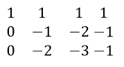
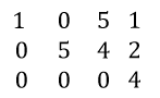
- Make an augmented matrix from the matrix ‘A’ and ‘Z’.

What I have done is I have just concatenated the two matrices. The augmented matrix simply tells that the elements in a row are coefficients of ‘x’, ‘y’ and ‘z’ and last element in the row is right-hand side of the equation.
- Multiply row (1) with 2 and subtract from row (2). Similarly, multiply equation 1 with 5 and subtract from row (3).
- In order to make an upper triangular matrix, multiply row (2) by 2 and then subtract from row (3).
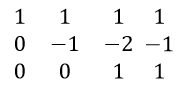
Remember to make each leading coefficient, also called pivot equal to 1, by suitable manipulations; in this case multiplying row 2 with -1. Also, if a row consists of 0 only, it should be below each row which consists of a non-zero entry. The resulting form of Matrix is called Row Echelon form. Notice that the planes corresponding to new equations formed by manipulation are not equivalent. Doing these operations, we are just conserving the solution of equations and trying to reach to it.
- Now we have simplified our job, let’s retrieve the modified equations. We will start from the simplest i.e. the one with the minimum number of remaining variables. If you follow the illustrated procedure, you will find that last equation comes to be the simplest one.
0*x+0*y+1*z=1
z=1
Now retrieve equation (2) and put the value of ‘z’ in it to find ‘y’. Do the same for equation (1).
Isn’t it pretty simple and clean?
Let’s ponder over another point. Will we always be able to make an upper triangular matrix which gives a unique solution? Are there different cases possible? Recall that planes can intersect in multiple ways. Take your time to figure it out and then proceed further.
Different possible cases-
- It’s possible that we get a unique solution as illustrated in above example. It indicates that all the three planes intersect in a point.
- We can get a case like shown below
Note that in last equation, 0=0 which is always true but it seems like we have got only 2 equations. One of the equations is redundant. In many cases, it’s also possible that the number of redundant equations is more than one. In this case, the number of solutions is infinite.
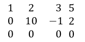
- There is another case where Echelon matrix looks as shown below
Let’s retrieve the last equation.
0*x+0*y+0*z=4
0=4
Is it possible? Very clear cut intuition is NO. But, does this signify something? It’s analogous to saying that it is impossible to find a solution and indeed, it is true. We can’t find a solution for such a set of equations. Can you think what is happening actually in terms of planes? Go back to the section where we saw planes intersecting and find it out.
Note that this method is efficient for a set of 5-6 equations. Although the method is quite simple, if equation set gets larger, the number of times you have to manipulate the equations becomes enormously high and the method becomes inefficient.
Rank of a matrix – Rank of a matrix is equal to the maximum number of linearly independent row vectors in a matrix.
A set of vectors is linearly dependent if we can express at least one of the vectors as a linear combination of remaining vectors in the set.
4.2 Inverse of a Matrix
For solving a large number of equations in one go, the inverse is used. Don’t panic if you are not familiar with the inverse. We will do a good amount of work on all the required concepts. Let’s start with a few terms and operations.
Determinant of a Matrix – The concept of determinant is applicable to square matrices only. I will lead you to the generalised expression of determinant in steps. To start with, let’s take a 2*2 matrix A.
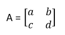
For now, just focus on 2*2 matrix. The expression of determinant of the matrix A will be:
det(A) =a*d-b*c
Note that det(A) is a standard notation for determinant. Notice that all you have to do to find determinant in this case is to multiply diagonal elements together and put a positive or negative sign before them. For determining the sign, sum the indices of a particular element. If the sum is an even number, put a positive sign before the multiplication and if the sum is odd, put a negative sign. For example, the sum of indices of element ‘a11’ is 2. Similarly the sum of indices of element ‘d’ is 4. So we put a positive sign before the first term in the expression. Do the same thing for the second term yourself.
Now take a 3*3 matrix ‘B’ and find its determinant.
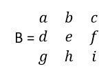
I am writing the expression first and then will explain the procedure step by step.

Each term consists of two parts basically i.e. a submatrix and a coefficient. First of all, pick a constant. Observe that coefficients are picked from the first row only. To start with, I have picked the first element of the first row. You can start wherever you want. Once you have picked the coefficient, just delete all the elements in the row and column corresponding to the chosen coefficient. Next, make a matrix of the remaining elements; each one in its original position after deleting the row and column and find the determinant of this submatrix . Repeat the same procedure for each element in the first row. Now, for determining the sign of the terms, just add the indices of the coefficient element. If it is even, put a positive sign and if odd, put a negative sign. Finally, add all the terms to find the determinant. Now, let’s take a higher order matrix ‘C’ and generalise the concept.
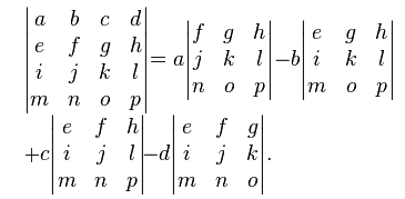
Try to relate the expression to what we have done already and figure out the final expression.
Code in python
import numpy as np
#create a 4*4 matrix
arr = np.arange(100,116).reshape(4,4)
#find the determinant
np.linalg.det(arr)
Code in R
[,1] [,2] [,3]
[1,] -0.16208333 -0.1125 0.17458333
[2,] -0.07916667 0.1250 -0.04583333
[3,] 0.20791667 -0.0125 -0.09541667

#Determinant
-0.0004166667
Minor of a matrix
Let’s take a square matrix A. then minor corresponding to an element A(ij) is the determinant of the submatrix formed by deleting the ‘i’th row and ‘j’th column of the matrix. Hope you can relate with what I have explained already in the determinant section. Let’s take an example.
To find the minor corresponding to element A11, delete first row and first column to find the submatrix.

Now find the determinant of this matrix as explained already. If you calculate the determinant of this matrix, you should get 4. If we denote minor by M11, then
M11 = 4
Similarly, you can do for other elements.
Cofactor of a matrix
In the above discussion of minors, if we consider signs of minor terms, the resultant we get is called cofactor of a matrix. To assign the sign, just sum the indices of the corresponding element. If it turns out to be even, assign positive sign. Else assign negative. Let’s take above illustration as an example. If we add the indices i.e. 1+1=2, so we should put a positive sign. Let’s say it C11. Then
C11 = 4
You should find cofactors corresponding to other elements by yourself for a good amount of practice.
Cofactor matrix
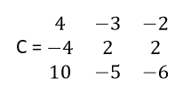
Find the cofactor corresponding to each element. Now in the original matrix, replace the original element by the corresponding cofactor. The matrix thus found is called the cofactor matrix corresponding to the original matrix.
For example, let’s take our matrix A. if you have found out the cofactors corresponding to each element, just put them in a matrix according to rule stated above. If you have done it right, you should get cofactor matrix
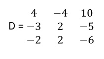
Adjoint of a matrix – In our journey to find inverse, we are almost at the end. Just keep hold of the article for a couple of minutes and we will be there. So, next we will find the adjoint of a matrix.
Suppose we have to find the adjoint of a matrix A. we will do it in two steps.
In step 1, find the cofactor matrix of A.
In step 2, just transpose the cofactor matrix.
The resulting matrix is the adjoint of the original matrix. For illustration, lets find the adjoint of our matrix A. we already have cofactor matrix C. Transpose of cofactor matrix should be
Finally, in the next section, we will find the inverse.
4.2.1 Finding Inverse of a matrix
Do you remember the concept of the inverse of a number in elementary algebra? Well, if there exist two numbers such that upon their multiplication gives 1 then those two numbers are called inverse of each other. Similarly in linear algebra, if there exist two matrices such that their multiplication yields an identity matrix then the matrices are called inverse of each other. If you can not get what I explained, just go with the article. It will come intuitively to you. The best way to learning is learning by doing. So, let’s jump straight to the algorithm for finding the inverse of a matrix A. Again, we will do it in two steps.
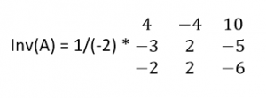
Step 1: Find out the adjoint of the matrix A by the procedure explained in previous sections.
Step2: Multiply the adjoint matrix by the inverse of determinant of the matrix A. The resulting matrix is the inverse of A.
For example, let’s take our matrix A and find it’s inverse. We already have the adjoint matrix. Determinant of matrix A comes to be -2. So, its inverse will be
Now suppose that the determinant comes out to be 0. What happens when we invert the determinant i.e. 0? Does it make any sense? It indicates clearly that we can’t find the inverse of such a matrix. Hence, this matrix is non-invertible. More technically, this type of matrix is called a singular matrix.
Keep in mind that the resultant of multiplication of a matrix and its inverse is an identity matrix. This property is going to be used extensively in equation solving.
Inverse is used in finding parameter vector corresponding to minimum cost function in linear regression.
4.2.2 Power of matrices
What happens when we multiply a number by 1? Obviously it remains the same. The same is applicable for an identity matrix i.e. if we multiply a matrix with an identity matrix of the same order, it remains same.
Lets solve our original problem with the help of matrices. Our original problem represented in matrix was as shown below
AX = Z i.e.
What happens when we pre multiply both the sides with inverse of coefficient matrix i.e. A. Lets find out by doing.
A-1 A X =A-1 Z
We can manipulate it as,
(A-1 A) X = A -1Z
But we know multiply a matrix with its inverse gives an Identity Matrix. So,
IX = A -1Z
Where I is the identity matrix of the corresponding order.
If you observe keenly, we have already reached to the solution. Multiplying identity matrix to X does not change it. So the equation becomes
X = A -1Z
For solving the equation, we have to just find the inverse. It can be very easily done by executing a few lines of codes. Isn’t it a really powerful method?
Code for inverse in python
import numpy as np
#create an array arr1
arr1 = np.arange(5,21).reshape(4,4)
#find the inverse
np.linalg.inv(arr1)
4.2.3 Application of inverse in Data Science
Inverse is used to calculate parameter vector by normal equation in linear equation. Here is an illustration. Suppose we are given a data set as shown below-
| Team | League | Year | RS | RA | W | OBP | SLG | BA | G | OOBP | OSLG |
| ARI | NL | 2012 | 734 | 688 | 81 | 0.328 | 0.418 | 0.259 | 162 | 0.317 | 0.415 |
| ATL | NL | 2012 | 700 | 600 | 94 | 0.32 | 0.389 | 0.247 | 162 | 0.306 | 0.378 |
| BAL | AL | 2012 | 712 | 705 | 93 | 0.311 | 0.417 | 0.247 | 162 | 0.315 | 0.403 |
| BOS | AL | 2012 | 734 | 806 | 69 | 0.315 | 0.415 | 0.26 | 162 | 0.331 | 0.428 |
| CHC | NL | 2012 | 613 | 759 | 61 | 0.302 | 0.378 | 0.24 | 162 | 0.335 | 0.424 |
| CHW | AL | 2012 | 748 | 676 | 85 | 0.318 | 0.422 | 0.255 | 162 | 0.319 | 0.405 |
| CIN | NL | 2012 | 669 | 588 | 97 | 0.315 | 0.411 | 0.251 | 162 | 0.305 | 0.39 |
| CLE | AL | 2012 | 667 | 845 | 68 | 0.324 | 0.381 | 0.251 | 162 | 0.336 | 0.43 |
| COL | NL | 2012 | 758 | 890 | 64 | 0.33 | 0.436 | 0.274 | 162 | 0.357 | 0.47 |
| DET | AL | 2012 | 726 | 670 | 88 | 0.335 | 0.422 | 0.268 | 162 | 0.314 | 0.402 |
| HOU | NL | 2012 | 583 | 794 | 55 | 0.302 | 0.371 | 0.236 | 162 | 0.337 | 0.427 |
| KCR | AL | 2012 | 676 | 746 | 72 | 0.317 | 0.4 | 0.265 | 162 | 0.339 | 0.423 |
| LAA | AL | 2012 | 767 | 699 | 89 | 0.332 | 0.433 | 0.274 | 162 | 0.31 | 0.403 |
| LAD | NL | 2012 | 637 | 597 | 86 | 0.317 | 0.374 | 0.252 | 162 | 0.31 | 0.364 |
It describes the different variables of different baseball teams to predict whether it makes to playoffs or not. But for right now to make it a regression problem, suppose we are interested in predicting OOBP from the rest of the variables. So, ‘OOBP’ is our target variable. To solve this problem using linear regression, we have to find parameter vector. If you are familiar with Normal equation method, you should have the idea that to do it, we need to make use of Matrices. Lets proceed further and denote our Independent variables below as matrix ‘X’.This data is a part of a data set taken from analytics edge. Here is the link for the data set.
so, X=
| 734 | 688 | 81 | 0.328 | 0.418 | 0.259 |
| 700 | 600 | 94 | 0.32 | 0.389 | 0.247 |
| 712 | 705 | 93 | 0.311 | 0.417 | 0.247 |
| 734 | 806 | 69 | 0.315 | 0.415 | 0.26 |
| 613 | 759 | 61 | 0.302 | 0.378 | 0.24 |
| 748 | 676 | 85 | 0.318 | 0.422 | 0.255 |
| 669 | 588 | 97 | 0.315 | 0.411 | 0.251 |
| 667 | 845 | 68 | 0.324 | 0.381 | 0.251 |
| 758 | 890 | 64 | 0.33 | 0.436 | 0.274 |
| 726 | 670 | 88 | 0.335 | 0.422 | 0.268 |
| 583 | 794 | 55 | 0.302 | 0.371 | 0.236 |
| 676 | 746 | 72 | 0.317 | 0.4 | 0.265 |
| 767 | 699 | 89 | 0.332 | 0.433 | 0.274 |
| 637 | 597 | 86 | 0.317 | 0.374 | 0.252 |
To find the final parameter vector(θ) assuming our initial function is parameterised by θ and X , all you have to do is to find the inverse of (XT X) which can be accomplished very easily by using code as shown below.
First of all, let me make the Linear Regression formulation easier for you to comprehend.
f θ (X)= θT X, where θ is the parameter we wish to calculate and X is the column vector of features or independent variables.
import pandas as pd
import numpy as np
#you don’t need to bother about the following. It just #transforms the data from original source into matrix
Df = pd.read_csv( "../baseball.csv”)
Df1 = df.head(14)
# We are just taking 6 features to calculate θ.
X = Df1[[‘RS’, ‘RA’, ‘W’, ‘OBP’,'SLG','BA']]
Y=Df1['OOBP']
#Converting X to matrix
X = np.asmatrix(X)
#taking transpose of X and assigning it to x
x= np.transpose(X)
#finding multiplication
T= x.dot(X)
#inverse of T - provided it is invertible otherwise we use pseudoinverse
inv=np.linalg.inv(T)
#calculating θ
theta=(inv.dot(X.T)).dot(Y)
Imagine if you had to solve this set of equations without using linear algebra. Let me remind you that this data set is less than even 1% of original date set. Now imagine if you had to find parameter vector without using linear algebra. It would have taken a lots of time and effort and could be even impossible to solve sometimes.
One major drawback of normal equation method when the number of features is large is that it is computationally very costly. The reason is that if there are ‘n’ features, the matrix (XT X) comes to be the order n*n and its solution costs time of order O( n*n*n). Generally, normal equation method is applied when a number of features is of the order of 1000 or 10,000. Data sets with a larger number of features are handled with the help another method called Gradient Descent.
Next, we will go through another advanced concept of linear algebra called Eigenvectors.
5. Eigenvalues and Eigenvectors
Eigenvectors find a lot of applications in different domains like computer vision, physics and machine learning. If you have studied machine learning and are familiar with Principal component analysis algorithm, you must know how important the algorithm is when handling a large data set. Have you ever wondered what is going on behind that algorithm? Actually, the concept of Eigenvectors is the backbone of this algorithm. Let us explore Eigen vectors and Eigen values for a better understanding of it.
Let’s multiply a 2-dimensional vector with a 2*2 matrix and see what happens.
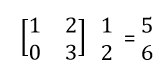
This operation on a vector is called linear transformation. Notice that the directions of input and output vectors are different. Note that the column matrix denotes a vector here.
I will illustrate my point with the help of a picture as shown below.
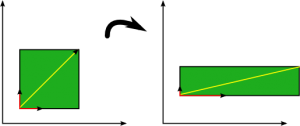
In the above picture, there are two types of vectors coloured in red and yellow and the picture is showing the change in vectors after a linear transformation. Note that on applying a linear transformation to yellow coloured vector, its direction changes but the direction of the red coloured vector doesn’t change even after applying the linear transformation. The vector coloured in red is an example of Eigenvector.
Precisely, for a particular matrix; vectors whose direction remains unchanged even after applying linear transformation with the matrix are called Eigenvectors for that particular matrix. Remember that the concept of Eigen values and vectors is applicable to square matrices only. Another thing to know is that I have taken a case of two-dimensional vectors but the concept of Eigenvectors is applicable to a space of any number of dimensions.
5.1 How to find Eigenvectors of a matrix?
Suppose we have a matrix A and an Eigenvector ‘x’ corresponding to the matrix. As explained already, after multiplication with matrix the direction of ‘x’ doesn’t change. Only change in magnitude is permitted. Let us write it as an equation-
Ax = cx
(A-c)x = 0 …….(1)
Please note that in the term (A-c), ‘c’ denotes an identity matrix of the order equal to ‘A’ multiplied by a scalar ‘c’
We have two unknowns ‘c’ and ‘x’ and only one equation. Can you think of a trick to solve this equation?
In equation (1), if we put the vector ‘x’ as zero vector, it makes no sense. Hence, the only choice is that (A-c) is a singular matrix. And singular matrix has a property that its determinant equals to 0. We will use this property to find the value of ‘c’.
Det(A-c) = 0
Once you find the determinant of the matrix (A-c) and equate to 0, you will get an equation in ‘c’ of the order depending upon the given matrix A. all you have to do is to find the solution of the equation. Suppose that we find solutions as ‘c1’ , ‘c2’ and so on. Put ‘c1’ in equation (1) and find the vector ‘x1’ corresponding to ‘c1’. The vector ‘x1’ that you just found is an Eigenvector of A. Now, repeat the same procedure with ‘c2’, ‘c3’ and so on.
Code for finding EigenVectors in python
import numpy as np
#create an array
arr = np.arange(1,10).reshape(3,3)
#finding the Eigenvalue and Eigenvectors of arr
np.linalg.eig(arr)
Code in R for finding Eigenvalues and Eigenvectors:
Output
147.737576 5.317459 -3.055035
[,1] [,2] [,3]
[1,] -0.3948374 0.4437557 -0.74478185
[2,] -0.5497457 -0.8199420 -0.06303763
[3,] -0.7361271 0.3616296 0.66432391
5.2 Use of Eigenvectors in Data Science
The concept of Eigenvectors is applied in a machine learning algorithm Principal Component Analysis. Suppose you have a data with a large number of features i.e. it has a very high dimensionality. It is possible that there are redundant features in that data. Apart from this, a large number of features will cause reduced efficiency and more disk space. What PCA does is that it craps some of lesser important features. But how to determine those features? Here, Eigenvectors come to our rescue.Let’s go through the algorithm of PCA. Suppose we have an ‘n’ dimensional data and we want to reduce it to ‘k’ dimensions. We will do it in steps.
Step 1: Data is mean normalised and feature scaled.
Step 2: We find out the covariance matrix of our data set.
Now we want to reduce the number of features i.e. dimensions. But cutting off features means loss of information. We want to minimise the loss of information i.e. we want to keep the maximum variance. So, we want to find out the directions in which variance is maximum. We will find these directions in the next step.
Step 3: We find out the Eigenvectors of the covariance matrix. You don’t need to bother much about covariance matrix. It’s an advanced concept of statistics. As we have data in ‘n’ dimensions, we will find ‘n’ Eigenvectors corresponding to ‘n’ Eigenvalues.
Step 4: We will select ‘k’ Eigenvectors corresponding to the ‘k’ largest Eigenvalues and will form a matrix in which each Eigenvector will constitute a column. We will call this matrix as U.
Now it’s the time to find the reduced data points. Suppose you want to reduce a data point ‘a’ in the data set to ‘k’ dimensions. To do so, you have to just transpose the matrix U and multiply it with the vector ‘a’. You will get the required vector in ‘k’ dimensions.
Once we are done with Eigenvectors, let’s talk about another advanced and highly useful concept in Linear algebra called Singular value decomposition, popularly called as SVD. Its complete understanding needs a rigorous study of linear algebra. In fact, SVD is a complete blog in itself. We will come up with another blog completely devoted to SVD. Stay tuned for a better experience. For now, I will just give you a glimpse of how SVD helps in data science.
6. Singular Value Decomposition
Suppose you are given a feature matrix A. As suggested by name, what we do is we decompose our matrix A in three constituent matrices for a special purpose. Sometimes, it is also said that svd is some sort of generalisation of Eigen value decomposition. I will not go into its mathematics for the reason already explained and will stick to our plan i.e. use of svd in data science.
Svd is used to remove the redundant features in a data set. Suppose you have a data set which comprises of 1000 features. Definitely, any real data set with such a large number of features is bound to contain redundant features. if you have run ML, you should be familiar with the fact that Redundant features cause a lots of problems in running machine learning algorithms. Also, running an algorithm on the original data set will be time inefficient and will require a lot of memory. So, what should you to do handle such a problem? Do we have a choice? Can we omit some features? Will it lead to significant amount of information loss? Will we be able to get an efficient enough algorithm even after omitting the rows? I will answer these questions with the help of an illustration.
Look at the pictures shown below taken from this link

We can convert this tiger into black and white and can think of it as a matrix whose elements represent the pixel intensity as relevant location. In simpler words, the matrix contains information about the intensity of pixels of the image in the form of rows and columns. But, is it necessary to have all the columns in the intensity matrix? Will we be able to represent the tiger with a lesser amount of information? The next picture will clarify my point. In this picture, different images are shown corresponding to different ranks with different resolution. For now, just assume that higher rank implies the larger amount of information about pixel intensity. The image is taken from this link

It is clear that we can reach to a pretty well image with 20 or 30 ranks instead of 100 or 200 ranks and that’s what we want to do in a case of highly redundant data. What I want to convey is that to get a reasonable hypothesis, we don’t have to retain all the information present in the original dataset. Even, some of the features cause a problem in reaching a solution to the best algorithm. For the example, presence of redundant features causes multi co-linearity in linear regression. Also, some features are not significant for our model. Omitting these features helps to find a better fit of algorithm along with time efficiency and lesser disk space. Singular value decomposition is used to get rid of the redundant features present in our data.
7. End notes
If you have made this far – give yourself a pat at the back. We have covered different aspects of Linear algebra in this article. I have tried to give sufficient amount of information as well as keep the flow such that everybody can understand the concepts and be able to do necessary calculations. Still, if you get stuck somewhere, feel free to comment below or post on discussion portal.


Great article Vikas! Can you please write an article on how SVD is used in recommendation system!
thanks Nikhil ! we will be coming up with a article on SVD in near future. Stay tuned.
Excellent article. It improved my understanding of solving linear equations using matrix by a great extent.
Thanks Aanish!
Good job Vikas
thanks Yuriy !