A Beginner-Friendly Guide to PyTorch and How it Works from Scratch

Overview

• What is PyTorch? How can you get started with it from scratch? We’ll cover all of that in this article
• PyTorch is one of the most popular deep learning libraries right now
• We’ll also take up a case study and use PyTorch to understand its practice applications

 

Introduction

Every once in a while, there comes a library or framework that reshapes and reimagines how we look at the field of deep learning. The remarkable progress a single framework can bring about never ceases to amaze me.

I can safely say PyTorch is on that list of deep learning frameworks. It has helped accelerate the research that goes into deep learning models by making them computationally faster and less expensive (a data scientist’s dream!).

I’ve personally found PyTorch really useful for my work. I delve heavily into the arts of computer vision and find myself leaning on PyTorch’s flexibility and efficiency quite often.

So in this article, I will guide you on how PyTorch works, and how you can get started with it today itself. We’ll cover everything there is to cover about this game-changing deep learning framework and also take up a really cool case study to see PyTorch in action.

Part II and III of this series are now live, and you can access them here:

• Build an Image Classification Model using Convolutional Neural Networks in PyTorch
• 
  

  Deep Learning for Everyone: Master the Powerful Art of Transfer Learning using PyTorch

  
  

If you prefer to approach learning PyTorch and the below concepts in a structured format, you can enrol for this free course and follow the concepts chapter-wise: PyTorch Course

 

Table of Contents

1. Getting Started with PyTorch
2. Basics of PyTorch
   1. Introduction to Tensors
   2. Mathematical Operations
   3. Matrix Initialization and Matrix Operations
3. Common PyTorch Modules
   1. Autograd
   2. Optim
   3. nn
4. Building a Neural Network from Scratch in PyTorch
5. Solving an Image Classification Problem using PyTorch
6. What’s Next?

 

Getting Started with PyTorch

PyTorch is a Python-based library that provides maximum flexibility and speed.

I’ve found PyTorch to be as simple as working with NumPy – and trust me, that is not an exaggeration.

You will figure this out really soon as we move forward in this article. But before we dive into the nuances of PyTorch, let’s look at some of the key features of this framework which make it unique and easy to use.

 

TorchScript

PyTorch TorchScript helps to create serializable and optimizable models. Once we train these models in Python, they can be run independently from Python as well. This helps when we’re in the model deployment stage of a data science project.

So, you can train a model in PyTorch using Python and then export the model via TorchScript to a production environment where Python is not available. We will discuss model deployment in more detail in the later articles of this series.

 

Distributed Training

PyTorch also supports distributed training which enables researchers as well as practitioners to parallelize their computations. Distributed training makes it possible to use multiple GPUs to process larger batches of input data. This, in turn, reduces the computation time.

 

Python Support

PyTorch has a very good interaction with Python. In fact, coding in PyTorch is quite similar to Python. So if you are comfortable with Python, you are going to love working with PyTorch.

 

Dynamic Computation Graphs

PyTorch has a unique way of building neural networks. It creates dynamic computation graphs meaning that the graph will be created on the fly:

And this is just skimming the surface of why PyTorch has become such a beloved framework in the data science community.

Right – now it’s time to get started with understanding the basics of PyTorch. So make sure you install PyTorch on your machine before proceeding. The latest version of PyTorch (PyTorch 1.2) was released on August 08, 2019 and you can see the installation steps for it using this link.

 

Basics of PyTorch

Remember how I said PyTorch is quite similar to Numpy earlier? Let’s build on that statement now. I will demonstrate basic PyTorch operations and show you how similar they are to NumPy.

In the NumPy library, we have multi-dimensional arrays whereas in PyTorch, we have tensors. So, let’s first understand what tensors are.

 

Introduction to Tensors

Tensors are multidimensional arrays. And PyTorch tensors are similar to NumPy’s n-dimensional arrays. We can use these tensors on a GPU as well (this is not the case with NumPy arrays). This is a major advantage of using tensors.

PyTorch supports multiple types of tensors, including:

1. FloatTensor: 32-bit float
2. DoubleTensor: 64-bit float
3. HalfTensor: 16-bit float
4. IntTensor: 32-bit int
5. LongTensor: 64-bit int

Now, let’s look at the basics of PyTorch along with how it compares against NumPy. If you are familiar with other deep learning frameworks, you must have come across tensors in TensorFlow as well. In fact, you are welcome to implement the following tasks in Tensorflow too and make your own comparison of PyTorch vs. TensorFlow!

We’ll start by importing both the NumPy and the Torch libraries:

	# importing libraries
	import numpy as np
	import torch

view raw library.py hosted with ❤ by GitHub

Now, let’s see how we can assign a variable in NumPy as well as PyTorch:

	# initializing a numpy array
	a = np.array(1)
	# initializing a tensor
	b = torch.tensor(1)
	print(a)
	print(b)

view raw assigning_variable.py hosted with ❤ by GitHub

 

 

Let’s quickly look at the type of both these variables:

type(a), type(b)

view raw type.py hosted with ❤ by GitHub

 

Type here confirms that the first variable (a) here is a NumPy array whereas the second variable (b) is a torch tensor.

Next, we will see how to perform mathematical operations on these tensors and how it is similar to NumPy’s mathematical operations.

 

Mathematical operations

Do you remember how to perform mathematical operations on NumPy arrays? If not, let me quickly recap that for you.

We will initialize two arrays and then perform mathematical operations like addition, subtraction, multiplication, and division, on them:

import numpy as np
# initializing two arrays
a = np.array(2)
b = np.array(1)
print(a,b)

These are the two NumPy arrays we have initialized. Now let’s see how we can perform mathematical operations on these arrays:

	# addition
	print(a+b)
	# subtraction
	print(b-a)
	# multiplication
	print(a*b)
	# division
	print(a/b)

view raw mathematical_operation_numpy.py hosted with ❤ by GitHub

 

 

Let’s now see how we can do the same using PyTorch on tensors. So, first, let’s initialize two tensors:

	# initializing two tensors
	a = torch.tensor(2)
	b = torch.tensor(1)
	print(a,b)

view raw tensor.py hosted with ❤ by GitHub

 

Next, perform the operations which we saw in NumPy:

	# addition
	print(a+b)
	# subtraction
	print(b-a)
	# multiplication
	print(a*b)
	# division
	print(a/b)

view raw mathematical_operation_torch.py hosted with ❤ by GitHub

 

 

Did you see the similarities? The codes are exactly the same to perform the above mentioned mathematical operations in both NumPy and PyTorch.

Next, let’s see how to initialize a matrix as well as perform matrix operations in PyTorch (along with, you guessed it, it’s NumPy counterpart!).

 

Matrix Initialization

Let’s say we want a matrix of shape 3*3 having all zeros. Take a moment to think – how can we do that using NumPy?

	# matrix of zeros
	a = np.zeros((3,3))
	print(a)
	print(a.shape)

view raw matrix_numpy.py hosted with ❤ by GitHub

 

 

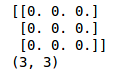
Fairly straightforward. We just have to use the zeros() function of NumPy and pass the desired shape ((3,3) in our case), and we get a matrix consisting of all zeros. Let’s now see how we can do this in PyTorch:

	# matrix of zeros
	a = torch.zeros((3,3))
	print(a)
	print(a.shape)

view raw matrix_zero.py hosted with ❤ by GitHub

 

 

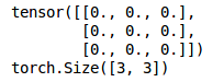
Similar to NumPy, PyTorch also has the zeros() function which takes the shape as input and returns a matrix of zeros of a specified shape. Now, while building a neural network, we randomly initialize the weights for the model. So, let’s see how we can initialize a matrix with random numbers:

	# setting the random seed for numpy
	np.random.seed(42)
	# matrix of random numbers
	a = np.random.randn(3,3)
	a

view raw random_matrix_numpy.py hosted with ❤ by GitHub

 

 

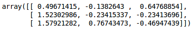
We have specified the random seed at the beginning here so that every time we run the above code, the same random number will generate. The random.randn() function returns random numbers that follow a standard normal distribution.

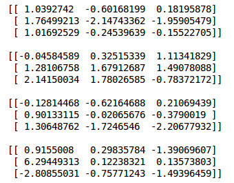
But let’s not get waylaid by the statistics part of things. We’ll focus on how we can initialize a similar matrix of random numbers using PyTorch:

 

 

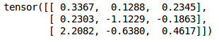
This is where even more similarities with NumPy crop up. PyTorch also has a function called randn() that returns a tensor filled with random numbers from a normal distribution with mean 0 and variance 1 (also called the standard normal distribution).

Note that we have set the random seed here as well just to reproduce the results every time you run this code. So far, we have seen how to initialize a matrix using PyTorch. Next, let’s see how to perform matrix operations in PyTorch.

 

Matrix Operations

We will first initialize two matrices in NumPy:

	# setting the random seed for numpy and initializing two matrices
	np.random.seed(42)
	a = np.random.randn(3,3)
	b = np.random.randn(3,3)

view raw random_numpy.py hosted with ❤ by GitHub

Next, let’s perform basic operations on them using NumPy:

	# matrix addition
	print(np.add(a,b), '\n')
	# matrix subtraction
	print(np.subtract(a,b), '\n')
	# matrix multiplication
	print(np.dot(a,b), '\n')
	# matrix multiplication
	print(np.divide(a,b))

view raw matrix_operation_numpy.py hosted with ❤ by GitHub

 

 

 

 

 

 

 

Matrix transpose is one technique which is also very useful while creating a neural network from scratch. So let’s see how we take the transpose of a matrix in NumPy:

	# original matrix
	print(a, '\n')
	# matrix transpose
	print(np.transpose(a))

view raw transpose_numpy.py hosted with ❤ by GitHub

 

 

 

 

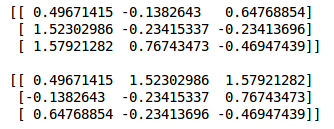
The transpose() function of NumPy automatically returns the transpose of a matrix. How does this happen in PyTorch? Let’s find out:

	# setting the random seed for pytorch and initializing two tensors
	torch.manual_seed(42)
	a = torch.randn(3,3)
	b = torch.randn(3,3)

view raw random_tensor.py hosted with ❤ by GitHub

 

 

 

 

 

 

 

Note that the .mm() function of PyTorch is similar to the dot product in NumPy. This function will be helpful when we create our model from scratch in PyTorch. Calculating transpose is also similar to NumPy:

	# original matrix
	print(a, '\n')
	# matrix transpose
	torch.t(a)

view raw transpose_torch.py hosted with ❤ by GitHub

 

 

 

 

Next, we will look at some other common operations like concatenating and reshaping tensors. From this point forward, I will not be comparing PyTorch against NumPy as you must have got an idea of how the codes are similar.

 

Concatenating Tensors

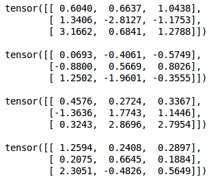
Let’s say we have two tensors as shown below:

	# initializing two tensors
	a = torch.tensor([[1,2],[3,4]])
	b = torch.tensor([[5,6],[7,8]])
	print(a, '\n')
	print(b)

view raw initialize_torch.py hosted with ❤ by GitHub

 

 

 

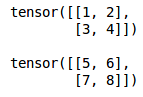
What if we want to concatenate these tensors vertically? We can use the below code:

 

 

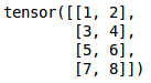
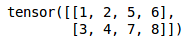
As you can see, the second tensor has been stacked below the first tensor. We can concatenate the tensors horizontally as well by setting the dim parameter to 1:

	# concatenating horizontally
	torch.cat((a,b),dim=1)

view raw concate_h_torch.py hosted with ❤ by GitHub

 

 

 

Reshaping Tensors

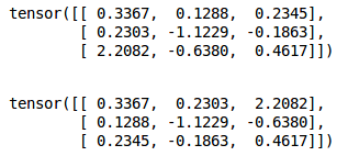
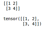
Let’s say we have the following tensor:

 

 

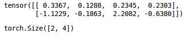
We can use the .reshape() function and pass the required shape as a parameter. Let’s try to convert the above tensor of shape (2,4) to a tensor of shape (1,8):

	# reshaping tensor
	b = a.reshape(1,8)
	print(b)
	b.shape

view raw reshape_tensor.py hosted with ❤ by GitHub

 

 

Awesome! PyTorch also provides the functionality to convert NumPy arrays to tensors. You can use the below code to do it:

	# initializing a numpy array
	a = np.array([[1,2],[3,4]])
	print(a, '\n')
	# converting the numpy array to tensor
	tensor = torch.from_numpy(a)
	print(tensor)

view raw convert_array_to_tensor.py hosted with ❤ by GitHub

 

 

 

With me so far? Good – let’s move on and dive deeper into the various aspects of PyTorch.

 

Common PyTorch Modules

Autograd Module

PyTorch uses a technique called automatic differentiation. It records all the operations that we are performing and replays it backward to compute gradients. This technique helps us to save time on each epoch as we are calculating the gradients on the forward pass itself.

Let’s look at an example to understand how the gradients are computed:

	# initializing a tensor
	a = torch.ones((2,2), requires_grad=True)
	a

view raw tensor_init.py hosted with ❤ by GitHub

 

 

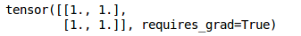
Here, we have initialized a tensor. Specifying requires_grad as True will make sure that the gradients are stored for this particular tensor whenever we perform some operation on it. Let’s now perform some operations on the defined tensor:

	# performing operations on the tensor
	b = a + 5
	c = b.mean()
	print(b,c)

view raw tensor_operation.py hosted with ❤ by GitHub

 

 

First of all, we added 5 to all the elements of this tensor and then taken the mean of that tensor. We will first manually calculate the gradients and then verify that using PyTorch. We performed the following operations on a:

b = a + 5

c = mean(b) = Σ(a+5) / 4

Now, the derivative of c w.r.t. a will be ¼ and hence the gradient matrix will be 0.25. Let’s verify this using PyTorch:

	# back propagating
	c.backward()
	# computing gradients
	print(a.grad)

view raw backprop.py hosted with ❤ by GitHub

 

 

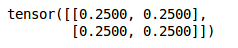
As expected, we have the gradients.

The autograd module helps us to compute the gradients in the forward pass itself which saves a lot of computation time of an epoch.

 

Optim Module

The Optim module in PyTorch has pre-written codes for most of the optimizers that are used while building a neural network. We just have to import them and then they can be used to build models.

Let’s see how we can use an optimizer in PyTorch:

	# importing the optim module
	from torch import optim
	# adam
	## adam = optim.Adam(model.parameters(), lr=learning_rate)
	# sgd
	## SGD = optim.SGD(model.parameters(), lr=learning_rate)

view raw optim.py hosted with ❤ by GitHub

Above are the examples to get the ADAM and SGD optimizers. Most of the commonly used optimizers are supported in PyTorch and hence we do not have to write them from scratch. Some of them are:

• SGD
• Adam
• Adadelta
• Adagrad
• AdamW
• SparseAdam
• Adamax
• ASGD (Averaged Stochastic Gradient Descent)
• RMSprop
• Rprop (resilient backpropagation)

 

nn Module

The autograd module in PyTorch helps us define computation graphs as we proceed in the model. But, just using the autograd module can be low-level when we are dealing with a complex neural network.

In those cases, we can make use of the nn module. This defines a set of functions, similar to the layers of a neural network, which takes the input from the previous state and produces an output.

We will use all these modules and define our neural network to solve a case study in the later sections. For now, let’s build a neural network from scratch that will help us understand how PyTorch works in a practical way.

 

Building a Neural Network from Scratch in PyTorch

I hope you are comfortable with building a neural network from scratch using NumPy. If not, I highly recommend you go through this article.

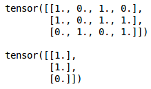
Alright – time to get started with neural networks! This is going to be a lot of fun so let’s get right down to it. We will first initialize the input and output:

	#Input tensor
	X = torch.Tensor([[1,0,1,0],[1,0,1,1],[0,1,0,1]])
	#Output
	y = torch.Tensor([[1],[1],[0]])
	print(X, '\n')
	print(y)

view raw input_output_tensor.py hosted with ❤ by GitHub

 

 

 

 

Next, we will define the sigmoid function which will act as the activation function and the derivative of the sigmoid function which will help us in the backpropagation step:

	#Sigmoid Function
	def sigmoid (x):
	return 1/(1 + torch.exp(-x))
	#Derivative of Sigmoid Function/
	def derivatives_sigmoid(x):
	return sigmoid(x) * (1 - sigmoid(x))

view raw sigmoid.py hosted with ❤ by GitHub

Next, initialize the parameters for our model including the number of epochs, learning rate, weights, biases, etc.:

	#Variable initialization
	epoch=7000 #Setting training iterations
	lr=0.1 #Setting learning rate
	inputlayer_neurons = X.shape[1] #number of features in data set
	hiddenlayer_neurons = 3 #number of hidden layer neurons
	output_neurons = 1 #number of neurons in output layer
	#weight and bias initialization
	wh=torch.randn(inputlayer_neurons, hiddenlayer_neurons).type(torch.FloatTensor)
	bh=torch.randn(1, hiddenlayer_neurons).type(torch.FloatTensor)
	wout=torch.randn(hiddenlayer_neurons, output_neurons)
	bout=torch.randn(1, output_neurons)

view raw variable_initialization.py hosted with ❤ by GitHub

Here we have randomly initialized the weights and biases using the .randn() function which we saw earlier. Finally, we will create a neural network. I am taking a simple model here just to make things clear. There is a single hidden layer and an input and an output layer in the model:

	for i in range(epoch):
	#Forward Propogation
	hidden_layer_input1 = torch.mm(X, wh)
	hidden_layer_input = hidden_layer_input1 + bh
	hidden_layer_activations = sigmoid(hidden_layer_input)
	output_layer_input1 = torch.mm(hidden_layer_activations, wout)
	output_layer_input = output_layer_input1 + bout
	output = sigmoid(output_layer_input)
	#Backpropagation
	E = y-output
	slope_output_layer = derivatives_sigmoid(output)
	slope_hidden_layer = derivatives_sigmoid(hidden_layer_activations)
	d_output = E * slope_output_layer
	Error_at_hidden_layer = torch.mm(d_output, wout.t())
	d_hiddenlayer = Error_at_hidden_layer * slope_hidden_layer
	wout += torch.mm(hidden_layer_activations.t(), d_output) *lr
	bout += d_output.sum() *lr
	wh += torch.mm(X.t(), d_hiddenlayer) *lr
	bh += d_output.sum() *lr

view raw nn_pytorch_scratch.py hosted with ❤ by GitHub

In the forward propagation step, we are calculating the output and finally, in the backward propagation step, we are calculating the error. We will then update the weights and biases using this error.

Let’s now look at the output from the model:

	print('actual :\n', y, '\n')
	print('predicted :\n', output)

view raw nn_torch_prediction.py hosted with ❤ by GitHub

 

 

 

 

 

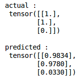
So, the target is 1, 1, 0 and the predicted values from the model are 0.98, 0.97 and 0.03. Not bad at all!

This is how we can build and train a neural network from scratch in PyTorch. Let’s now take things up a notch and dive into a case study. We will try to solve that case study using the techniques we have learned in this article.

 

Solving an Image Classification Problem using PyTorch

You’re going to love this section. This is where all our learning will culminate in a final neural network model on a real-world case study, and we will see how the PyTorch framework builds a deep learning model.

Our task is to identify the type of apparel by looking at a variety of apparel images. It’s a classic image classification problem using computer vision. This dataset, taken from the DataHack Platform, can be downloaded here.

There are a total of 10 classes in which we can classify the images of apparels:

Label	Description
0	T-shirt/top
1	Trouser
2	Pullover
3	Dress
4	Coat
5	Sandal
6	Shirt
7	Sneaker
8	Bag
9	Ankle boot

 

There are 70,000 images, out of which 60,000 are in the training set and the remaining 10,000 in the test set. All the images are grayscale images of size (28*28).

The dataset contains two folders – one each for the training set and the test set. In each folder, there is a .csv file that has the id of the image and its corresponding label and a folder containing the images for that particular set.

Loading the data

Let’s now get started with the code! We will first import the required libraries:

	# importing the libraries
	import pandas as pd
	import numpy as np
	from skimage.io import imread
	import matplotlib.pyplot as plt
	%matplotlib inline
	from sklearn.model_selection import train_test_split
	from sklearn.metrics import accuracy_score

view raw library_import.py hosted with ❤ by GitHub

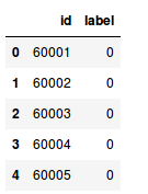
Next, read the .csv file that we downloaded from the competition page.

	# loading dataset
	train = pd.read_csv('train_LbELtWX/train.csv')
	test = pd.read_csv('test_ScVgIM0/test.csv')
	sample_submission = pd.read_csv('sample_submission_I5njJSF.csv')
	train.head()

view raw dataset.py hosted with ❤ by GitHub

 

 

 

 

 

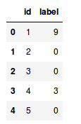
id here represents the name of the image (we just have to add .png as the images are in png format) and the label is the corresponding class of that particular image.

Let’s now plot an image to get a better understanding of how our data looks. We will randomly select an image and plot it. So, let’s first create a random number generator:

	# random number generator
	seed = 128
	rng = np.random.RandomState(seed)

view raw random_seed.py hosted with ❤ by GitHub

Plot an image:

	# print an image
	img_name = rng.choice(train['id'])
	filepath = 'train_LbELtWX/train/' + str(img_name) + '.png'
	img = imread(filepath, as_gray=True)
	img = img.astype('float32')
	plt.figure(figsize=(5,5))
	plt.imshow(img, cmap='gray')

view raw plot_image.py hosted with ❤ by GitHub

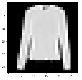
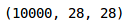
This is a random image from our dataset and gives us an idea of what all the other images look like. Next, we will load all the training images using the train.csv file. We will use a for loop to read all the images from the training set and finally store them as a NumPy array:

	# loading training images
	train_img = []
	for img_name in train['id']:
	image_path = 'train_LbELtWX/train/' + str(img_name) + '.png'
	img = imread(image_path, as_gray=True)
	img = img.astype('float32')
	train_img.append(img)
	train_x = np.array(train_img)
	train_x.shape

view raw train_images.py hosted with ❤ by GitHub

 

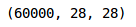
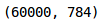
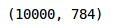
So, there are 60,000 images in the training set each of shape 28 x 28. We will be making a simple neural network which takes a one-dimensional input and hence we have to flatten these two-dimensional images into a single dimension:

	train_x = train_x/train_x.max()
	train_x = train_x.reshape(-1, 28*28).astype('float32')
	train_x.shape

view raw train_reshape.py hosted with ❤ by GitHub

 

We have reshaped the images to a single dimension. So far, we have created the input set but we also need the target to train the model, right? So, let’s go ahead and create that:

train_y = train['label'].values

view raw target.py hosted with ❤ by GitHub

Training the model

Let’s create a validation set to evaluate how well our model will perform on unseen data:

	# create validation set
	train_x, val_x, train_y, val_y = train_test_split(train_x, train_y, test_size = 0.1, stratify = train_y)
	(train_x.shape, train_y.shape), (val_x.shape, val_y.shape)

view raw validation_set.py hosted with ❤ by GitHub

 

We have taken 10 percent of the training data in the validation set.

Now, it’s time to define our model. We will first import the Torch package and the required modules:

	import torch
	from torch.autograd import Variable
	from torch.nn import Linear, ReLU, CrossEntropyLoss, Sequential
	from torch.optim import Adam

view raw torch_library.py hosted with ❤ by GitHub

Next, define the parameters like the number of neurons in the hidden layer, the number of epochs, and the learning rate:

	# number of neurons in each layer
	input_num_units = 28*28
	hidden_num_units = 500
	output_num_units = 10
	# set remaining variables
	epochs = 20
	learning_rate = 0.0005

view raw nn_parameters.py hosted with ❤ by GitHub

Finally, let’s build the model! For now, we will have a single hidden layer and choose the loss function as cross-entropy. We will be using the Adam optimizer here. Remember that there are other parameters of our model and you can change them as well.

	# define model
	model = Sequential(Linear(input_num_units, hidden_num_units),
	ReLU(),
	Linear(hidden_num_units, output_num_units))
	# loss function
	loss_fn = CrossEntropyLoss()
	# define optimization algorithm
	optimizer = Adam(model.parameters(), lr=learning_rate)

view raw model_torch.py hosted with ❤ by GitHub

Let’s now train the model for a specified number of epochs and save the training and validation loss for each epoch:

	train_losses = []
	val_losses = []
	for epoch in range(epochs):
	avg_cost = 0
	x, y = Variable(torch.from_numpy(train_x)), Variable(torch.from_numpy(train_y), requires_grad=False)
	x_val, y_val = Variable(torch.from_numpy(val_x)), Variable(torch.from_numpy(val_y), requires_grad=False)
	pred = model(x)
	pred_val = model(x_val)
	# get loss
	loss = loss_fn(pred, y)
	loss_val = loss_fn(pred_val, y_val)
	train_losses.append(loss)
	val_losses.append(loss_val)
	# perform backpropagation
	loss.backward()
	optimizer.step()
	avg_cost = avg_cost + loss.data
	if (epoch%2 != 0):
	print(epoch+1, avg_cost)

view raw model_training.py hosted with ❤ by GitHub

 

 

 

 

 

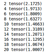
Here, I have printed the training losses after every second epoch and we can see that the loss is decreasing. Let’s now plot the training and validation loss to check whether they are in sync or not:

	# plotting the training and validation loss
	plt.plot(train_losses, label='Training loss')
	plt.plot(val_losses, label='Validation loss')
	plt.legend()
	plt.show()

view raw losses.py hosted with ❤ by GitHub

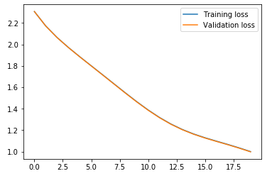
Perfect! We can see that the training and validation losses are in sync and the model is not overfitting. Let’s now check how accurate our model is on predicting the classes for both training and validation sets. We’ll start by looking at the training accuracy:

	# get training accuracy
	x, y = Variable(torch.from_numpy(train_x)), Variable(torch.from_numpy(train_y), requires_grad=False)
	pred = model(x)
	final_pred = np.argmax(pred.data.numpy(), axis=1)
	accuracy_score(train_y, final_pred)

view raw train_accuracy.py hosted with ❤ by GitHub

 

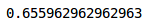
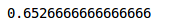
We got an accuracy of above 65% on the training set. Let’s check for the validation set as well:

	# get validation accuracy
	x, y = Variable(torch.from_numpy(val_x)), Variable(torch.from_numpy(val_y), requires_grad=False)
	pred = model(x)
	final_pred = np.argmax(pred.data.numpy(), axis=1)
	accuracy_score(val_y, final_pred)

view raw validation_accuracy.py hosted with ❤ by GitHub

 

We have an almost similar performance on the validation set. Note that even though we have used a very simple architecture with just one hidden layer, the performance is pretty good.

You can try to increase the number of hidden layers or play with other model parameters like the optimizer function, the number of hidden units, etc. and try to improve the performance further.

Getting predictions

Finally, let’s load the test images, make predictions on them and submit the predictions on the competition page. We will have to preprocess the test images in a similar way that we did for the training images:

	# loading test images
	test_img = []
	for img_name in test['id']:
	image_path = 'test_ScVgIM0/test/' + str(img_name) + '.png'
	img = imread(image_path, as_gray=True)
	img = img.astype('float32')
	test_img.append(img)
	test_x = np.array(test_img)
	test_x.shape

view raw test_images.py hosted with ❤ by GitHub

 

Let’s convert these images to a 1-d array now:

	# converting the images to 1-D
	test_x = test_x/train_x.max()
	test_x = test_x.reshape(-1, 28*28).astype('float32')
	test_x.shape

view raw test_reshape.py hosted with ❤ by GitHub

 

Finally, we will make predictions for these images:

	# getting the prediction for test images
	prediction = np.argmax(model(torch.from_numpy(test_x)).data.numpy(), axis=1)

view raw prediction.py hosted with ❤ by GitHub

Great, we now have the predictions. We will now save these predictions in the sample submission file:

	# first five rows of sample submission file
	sample_submission.head()

view raw sample_submission.py hosted with ❤ by GitHub

 

 

 

 

 

Replace these labels with the predictions that we got from the model for test images:

	# replacing the label with prediction
	sample_submission['label'] = prediction
	sample_submission.head()

view raw prediction_file.py hosted with ❤ by GitHub

 

 

 

 

 

Save this sample submission file and make a submission on the competition page:

	# saving the file
	sample_submission.to_csv('submission.csv', index=False)

view raw saving_prediction.py hosted with ❤ by GitHub

After submitting these predictions, we get an accuracy of 64.625% on the leaderboard. You can use this accuracy as a benchmark and try to improve on this by playing around with the parameters of the above model.

 

End Notes

In this article, we understood the basic concepts of PyTorch including how it’s quite intuitively similar to NumPy. We also saw how to build a neural network from scratch using.

We then took a case study where we solved an image classification problem and got a benchmark score of around 65% on the leaderboard. I encourage you to try and improve this score by changing different parameters of the model, including the optimizer function, increasing the number of hidden layers, tuning the number of hidden units, etc.

This article is the start of our journey with PyTorch. In the upcoming article, we will learn how to build convolutional neural networks in PyTorch, model checkpointing techniques, and how to deploy trained deep learning models using PyTorch. So stay tuned!

As always, if you have any doubts related to this article, feel free to post them in the comments section below. And make sure you check out our course if you’re interested in computer vision and deep learning:

• Computer Vision using Deep Learning 2.0