Overview
- Excel is the perfect fit for building your time series forecasting models
- We’ll discuss exponential smoothing models for time series forecasting, including the math behind them
- We’ll also implement these exponential smoothing models in MS Excel
Introduction
Time series in Excel – just seems like a natural fit, right? We see and design line charts in Excel all the time – from sales forecasts to revenue reviews – it all fits into how we think about using Excel in analytics and data science.
But here’s the thing about time series forecasting – it can appear daunting for beginners. It’s not a walk in the park. We need to understand how to deal with the time component and not just the other variables. And that time component can so often mess up our entire analysis!
While most courses and tutorials will show you how to perform time series forecasting in Python and R, this article has no such expectations. All you need is a working knowledge of Excel – and you’ll be able to follow along nicely!

So what are we going to cover in this article? We’ll talk about the concept of Exponential Smoothing Models for Time Series Forecasting, the maths involved, and show you how you can do exponential smoothing in MS Excel.
And if you’re new to Time Series forecasting and Excel, or need a refresher, we have these two popular free courses for you:
Table of Contents
- Introduction to Time Series Forecasting
- A Quick Look at the Different Time Series Components
- A List of Exponential Smoothing Models
- Simple Exponential Smoothing (with implementation in Excel)
- Double Exponential Smoothing (with implementation in Excel)
- Triple Exponential Smoothing (with implementation in Excel)
Introduction to Time Series Forecasting
We deal with time series data almost daily (without realizing it half the time). In our day to day lives, we often make conclusions about certain things based on our past observations and experiences.
For instance, if the stock price of a particular company has been dropping consistently over the last 10 days, we can assume that the price will drop tomorrow too. Or if it has been raining every day for the past week, we can guess that it would rain today as well, and hence it’s a good idea to carry an umbrella.
The above examples show that the recent past could give us a fair idea about the future. This is the main idea behind time series forecasting.
In a time series, each individual point is dependent on the previous value. Thus we can use past values and estimate the values in the future. The ‘time’ component is crucial here.
You can refer to the below article to know more about time series forecasting:
A Quick Look at the Different Time Series Components
To understand the exponential smoothing models and how they forecast future values, we must be familiar with the different time series components. A time series has the following three components:
-
Trend Component
The trend describes the general tendency of the data which could be increasing or decreasing or stable. For instance, at the time of demonetization, we observed a decreasing trend for stock prices. Or over the years, we have seen an increase in the number of sales of smartphones.
A trend often depicts the long term movement of the series. Have a look at the following examples – can you identify the trend in these series?
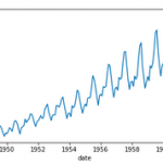
Even though there is some noise in the data, you can observe that there is an increasing trend in the above series.
-
Seasonal Component
The next important component is the seasonal component of the time series. For instance, there could be a higher sale in clothing items and sweets around New Year’s or Diwali every year. Similarly, there could be an increase in flight bookings around the holiday season(s). And this pattern could be observed throughout the year.
If you look closely at the images below, you would notice that there is a certain pattern that keeps repeating. This repeating pattern observed in the series is the seasonal component of the time series. It depicts the short term movement of the series.
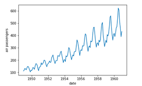
Although due to the noise in the series, you’ll notice that it’s slightly difficult to identify the seasonality in the first series. But the seasonality in the second series is evident. We have a particular pattern repeating every year, which shows that we have a yearly seasonality for the second series. If you explore the first series and take a closer look, you will find that it has a weekly seasonality.
-
Residual Component
Let’s say we identify the trend and seasonal component from a time series and remove these two. What remains after removing these two is the residual component. It does not have any pattern or trend. As the name suggests, the residual component is irregular.
So now that we understand the different components of a time series, let’s understand how exponential smoothing algorithms use these to make predictions.
A List of Exponential Smoothing Algorithms
Exponential smoothing algorithms are popularly used for forecasting univariate time series. Here are three types of exponential smoothing algorithms:
- Simple exponential smoothing
- Double exponential smoothing
- Triple exponential smoothing
We will learn about how each of these work, look into the mathematical equations for each, and implement these algorithms in Excel.
And here’s the problem statement we’ll be working on:
We are provided with the number of people who booked a JetRail on a given day. We need to forecast the number of bookings expected in the coming months. For more details on the problem statement, check out this link – Time Series Forecasting Practice Problem.
Simple Exponential Smoothing (with Implementation in Excel)
We know that the data points in a time series depend on each other. Hence, we can use historical data to make forecasts for the future.
Now, the question is – if you want to forecast the stock price for tomorrow, would you consider yesterday’s value or the price 10 days ago or last year?
Obviously yesterday’s price or last week’s value would give a better idea about the forecast than the values taken from a year ago. This implies that recency is an important factor in forecasting values. This is where exponential smoothing algorithms shine.
The simple exponential smoothing model considers the historical values and assigns weights to these values. The idea is that weights are higher for recent observations.
Let’s look at the mathematical equations for this:
Ŷt+1 = αYt + α(1-α)Yt-1 + α(1-α)2Yt-2 + α(1-α)3Yt-3 +…. .. .. (1)
Where,
- Yt represents the historical values
- Ŷt is the forecast
- alpha α is the smoothing parameter
The value of alpha (α) lies between 0-1. As you can see in the above equation, each subsequent Yt has a lower weight. Alpha is a hyperparameter and we can select the value of alpha. The table below will help you understand how changing the alpha value affects the forecasts:
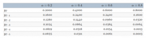
If the alpha value is low, more number of historical values are considered for the forecast. For higher values of alpha, such as 0.8 or 0.9, very few observations are taken into consideration.
Now, if we use the same equation for the second forecast, it will be:
Ŷt+2 = αYt+1 +α(1-α)Yt+ α(1-α)2Yt-1 + α(1-α)3Yt-2 + α(1-α)4Yt-3 +…. .. .. (2)
Similarly, we can write this equation for the remaining forecasts. You can see that each new term as an additional (1-alpha). The above equation can also be written as:
Ŷt+2 = αYt+1 +(1-α) [αYt+ α(1-α)1Yt-1 + α(1-α)2Yt-2 + α(1-α)3Yt-3 +….] .. .. (3)
If you compare the first and the third equation, you will find that the square brackets in this equation essentially have the LHS of the first equation. So we can simplify the third equation and write it as:
Ŷt+2 = αYt+1 +(1-α) [Ŷt+1] .. .. (4)
This is the simplified version of the simple exponential smoothing algorithm. For the subsequent forecast, we take into account the previously observed value and (1-alpha) times the previous forecast. This will save us a lot of calculations. We can undoubtedly use the expanded version, but that would increase the calculations.
Now that we have a good understanding of the above equations, let’s go ahead and use the equation to forecast the values and implement this in Excel.
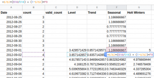
Step 1:
First, we do not have any historical values in step one. Hence, the first value is initialized manually. Here I have simply taken it to be the first observed value:
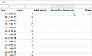
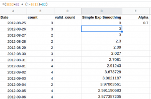
Step 2:
Then, for the next values, we have used equation (4) which we discussed above. You can see the same in the formula bar:
Note that here we are using the ‘observed value’ and making the predictions. When it comes to the test or validation set, we will not have any observed values, right? Then can we not make the predictions further? Let’s find out.
Step 3:
Since we do not have actual values for the test set (or validation set), we will use the last observed value as the actual value. Here is how we can do that:
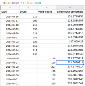
Check out the equation in the formula bar – we have fixed the Yt value. This is done using the $ sign with the column and the row value. So this is how you can make the prediction for the validation set. In this demonstration, I have fixed the alpha value as 0.7. Go ahead and try it out for different values of alpha and see how the result changes.
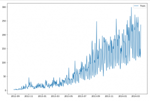
Here is the result of the forecasts. The yellow line is the forecast while blue and red lines are train and validation data:
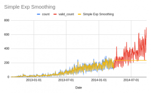
Notice that here we have a flat line. The simple exponential smoothing algorithm only considers the historical values but the trend component is not included in making the forecasts. This is resolved by the double exponential smoothing algorithm.
Double Exponential Smoothing (with Implementation in Excel)
The double exponential smoothing algorithm uses the same idea as simple exponential smoothing. It uses historical values for making the predictions and assigning the weights in an exponentially increasing manner (higher weight to the recent observations). Additionally, the double exponential smoothing also considers the ‘trend’ of the series.
Forecast (DES) = Level + Trend
‘Level’ here is the weighted average of the historical data, the same as we calculated for simple exponential smoothing. We can write the equation for Level as:
Lt+1 = αLt + (1-α) [L’t] .. .. (5)
This is similar to the simple exponential smoothing equation. The other component in the double exponential smoothing model is the ‘trend’. The ‘Trend’ is calculated as:
Tt+1 = β(Lt+1- Lt) + (1-β) Tt .. .. (6)
The beta here is a smoothing parameter for the trend component. The trend at a particular time is calculated to be the difference between the level terms (indicating an increase or decrease in the level). In order to consider the weighted sum of past trend values, we use (1-β) Tt where Tt is the trend calculated for the previous time step.
Now the final forecast will be Ŷt = Lt + Tt. Let’s find out how we can use these equations in Excel!
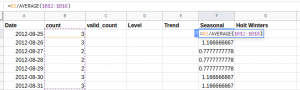
Step 1:
As we did before, since we do not have any historical values for step 1, we will have to initialize these values ourselves. Hence, initialize the first value manually.
Here, I have simply taken it to be the first observed value as the value for L1. The value for Trend (T1) is taken as 1.2 (you can change this value and see how the predictions vary).
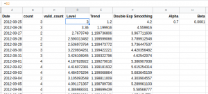
The smoothing parameter values are also defined at this point.
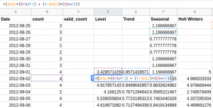
Step 2:
Then, for the next values, we will use the equation (5) and equation (6) which we discussed above. You can see the same in the formula bar.
Lt+1 = αLt + (1-α) [L’t] .. .. (5)
Tt+1 = β(Lt+1- Lt) + (1-β) Tt .. .. (6)
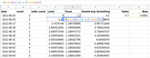
Like the previous example, here we are using the ‘observed value’, and making the predictions. For the validation or test set, we will not have any observed values. We will consider the last observed value throughout the validation set for making predictions.
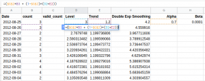
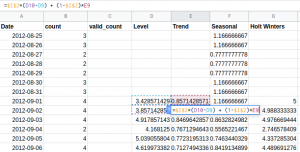
Step 3:
In the previous equations, we will replace the Lt and Tt for the validation set as the last observed value. The new forecasting equation becomes: Ŷt = Lt + hTt.
If the values of Lt and Tt are fixed, the forecast will be the same for all future points. Hence, to take into account the increasing trend, the coefficient ‘h’ is multiplied with the Trend component. The value of h is taken as 1,2,3, …..n for the next n forecasts:
See the equation in the formula bar – we have fixed the Lt and Tt values. Below is the result of the forecasts. The yellow line is the forecast while the blue and red lines are train and validation data:
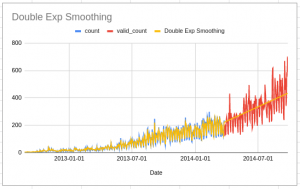
Notice that here we have an increasing line. The double exponential smoothing algorithm considers the trend and the historical values in making the forecasts.
Let’s look at the triple exponential smoothing model which also takes into account the seasonal component of the time series.
Triple Exponential Smoothing (with Implementation in Excel)
This is also popularly known as Holt Winter’s algorithm. The triple exponential smoothing algorithm, as you would have already guessed, considers three components – Level, Trend, and Seasonality.
Note that the seasonal component can be in the additive or multiplicative form. This means that the final forecast can be in either of the two forms:
Ŷt+1 = (Level + Trend) + Seasonality
Ŷt+1 = (Level + Trend) x Seasonality
Let’s look at the mathematical equations of each one of them and then we will use the multiplicative form in Excel to make the forecasts.
1. Triple Exponential Smoothing: Additive Seasonality
For forecasting the values, we will need to find the values of Level, Trend, and Seasonality. The equation of Level, in this case, has a seasonality adjusted observation (Yt – St-m), since we are adding the seasonal component for forecasting. Along with that, the calculation of Level includes the level and trend of previous observations:
Lt = α(Yt – St-m) + (1-α) [Lt-1 + Tt-1]
The equation of trend is the same as the double exponential smoothing model, given by:
Tt+1 = β(Lt+1- Lt) + (1-β) Tt
Finally, we need the equation of seasonality to make the forecasts. We have discussed the concept of seasonality in the previous sections. Seasonality is the repeating patterns observed in the series which can be useful for forecasting the values. For instance, in a weekly seasonality, the pattern will repeat every 7 days.
For capturing the seasonality, we take into consideration the previous nth value (and not the immediate value). Here is the equation for the additive seasonal component:
St = γ(Yt – Lt) + (1-γ)St-m
Gamma is the smoothing parameter for the seasonal component. Here, we consider the St-m, which is the seasonality at the previous mth time step. So, for a weekly seasonality, m = 7.
Now let us look at the multiplicative series for triple exponential smoothing.
2. Triple Exponential Smoothing: Multiplicative Seasonality
In this section, we will discuss the equations of level, trend, and seasonal component for multiplicative form and also use these to build a triple exponential smoothing model in Excel. We can calculate the level in the following manner:
Lt = α(Yt/ St-m) + (1-α)[Lt-1 + Tt-1 ]
Notice that the seasonal component is not subtracted, but divided here. The equation of trend is similar to the double exponential smoothing model. Here’s the equation:
Tt+1 = β(Lt+1- Lt) + (1-β) Tt
Finally, we have a seasonal component. This is the seasonal value at the particular time step t and the seasonal value at the t-m step. Here is how we can calculate the final value:
St = γ(Yt / Lt) + (1-γ)St-m
Food for thought – for the first time step, we don’t have the St-m value. Then how would we calculate the value of St? Well, we will have to initialize the values, as we did in the simple and double exponential smoothing models. Let’s have a look!
Step 1:
First, for the triple exponential smoothing algorithm, we have to initialize the values of the seasonal component. Since we have a weekly seasonality in this example, we have to initialize the first 7 values. These will be used for calculating the seasonal component for the series. You can initialize these values at your end.
Additionally, the first level and trend values are initialized in the following manner:
Lt = Yt/St-7
Tt = Lt – Lt-1
Once the required values are initialized, along with the alpha, beta, and gamma values, we can move to the next step. The alpha, beta, and gamma are hyperparameters and you can tune these values at your end to see how the results change. Here I have defined these values as:
![]()
Step 2:
So we have our initial values and the smoothing parameters in place. Now, we will be using the previously discussed equations for calculating the values of Level, Trend, and Seasonality.
The level at any time step is calculated as Lt = α(Yt/ St-m) + (1-α)[Lt-1 + Tt-1].
For the trend component, we will use the difference of Level at time steps t and t-1. In addition to this, the effect of previous time steps is taken with the weight of (1-β). Here is the equation: Tt+1 = β(Lt+1- Lt) + (1-β) Tt.
Finally, the seasonal component is: St = γ(Yt / Lt) + (1-γ)St-m.
And now we can make the final forecast using the below equation:
Ŷt+1 = (Lt + Tt) x St
Step 3:
These equations will work well for the training data, where we have the values of Yt which is used for calculating the level and the seasonal components. Making the forecasts for validation set (where Yt is not available) is slightly tricky.
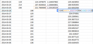
For determining the Level and trend values at the validation stage, we will use the same idea as implemented in double exponential smoothing. We will fix the value of Lt and Tt as the last calculated values. Furthermore, to include the increasing trend factor, we will use the coefficient h. But what about the seasonal (St) values? We will fix the last seven values of St.
The image below will help you understand the idea better:
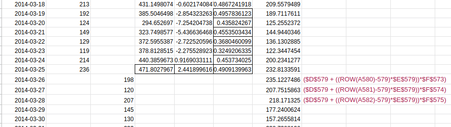
The validation set starts at 26-03-2014. Thus, the last observed level and trend values are at 25-03-2014. Also, the last seven seasonal component values are used to make the forecast for the next seven days. The same pattern is repeated for the remaining series.
Step 4:
Once the three components – Level, trend, and seasonal – are calculated, the final forecast will be:
Ŷt+1 = (Level + Trend) x Seasonality
Here is a plot that shows the actual values and forecasts:
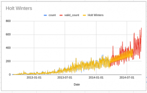
You can see that the forecasts, in this case, are significantly better than the previous two algorithms.
End Notes
Let’s summarize the copious amounts of learning we just did! We learned about the exponential smoothing models and how they work. We also implemented all of these models in Excel to understand the equations and calculations in detail.
Apart from these, there are various other time series algorithms that you can read about. Here are some resources to start you off:
-
7 methods to perform Time Series forecasting (with Python codes)
-
Build High-Performance Time Series Models using Auto ARIMA in Python and R
-
Generate Quick and Accurate Time Series Forecasts using Facebook’s Prophet (with Python & R codes)
Feel free to reach out to us in the comments section below in case you have any queries or feedback.
An avid reader and blogger who loves exploring the endless world of data science and artificial intelligence. Fascinated by the limitless applications of ML and AI; eager to learn and discover the depths of data science.


Hi, You have explained Time Series Analysis very well, in simple terms. Noted that in the model equations, squares & cubes are not 'super scripted', probably a printing error. Well done.
Hi, Thanks for sharing this model for stock price forecast on Excel. How would you take into consideration the feature of VOLUME as another criteria in your algorithm ? Thanks for sharing any idea. BR
Hi, Thanks for sharing this model on Excel. How would you take into consideration the volume of stock that is daily exchanged into your algorithm ? Much appreciated if you have any clue to plug this extra criteria to your model. BR