This article was published as a part of the Data Science Blogathon.
Hi everyone, for the past few months I am working on something called auto-encoders for Computer Vision and frankly I am impressed by the sheer number of applications that can be build using them. The purpose of this article is to explain about auto-encoders, some applications that you can build using auto-encoders, drawbacks of unconnected encoder-decoder layers, and how architectures like U-Net helps to improve the quality of an auto-encoder.
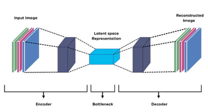
In simple words, an Auto-Encoder is a Sequential Neural Network that consists of two components an Encoder followed by a Decoder. For our reference let’s assume we are dealing with images, the job of an encoder is to extract features from the image, thereby reducing the image in height and width but simultaneously growing it in depth i.e an encoder makes a latent representation for the image. Now the job of the decoder is to decode the latent representation and form an image that satisfies our given criterion. This would be clear to understand from the following images.
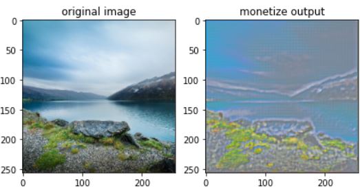
The input, as well as the output of an auto-encoder, is an image, in the example given below, the auto-encoder is converting the input to a Monet style painting.
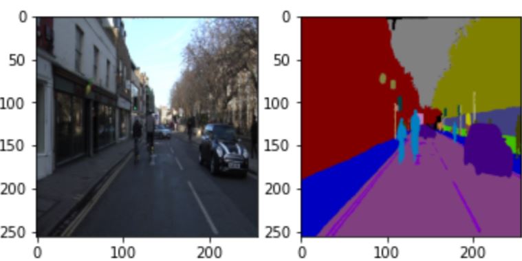
Semantic Segmentation refers to assigning a label to each pixel of an image thereby grouping the pixels that belong to the same object together, the following image will help you understand this better.
The following code defines the auto-encoder architecture used for this application:
myTransformer = tf.keras.models.Sequential([
## defining encoder
    tf.keras.layers.Input(shape= (256, 256, 3)),
    tf.keras.layers.Conv2D(filters = 16, kernel_size = (3,3), activation = 'relu', padding = 'same'),
    tf.keras.layers.MaxPool2D(pool_size = (2, 2)),
    tf.keras.layers.Conv2D(filters = 32, kernel_size = (3,3), strides = (2,2), activation = 'relu',
    padding = 'valid'),
    tf.keras.layers.Conv2D(filters = 64, kernel_size = (3,3), strides = (2,2), activation = 'relu',
    padding = 'same'),
    tf.keras.layers.MaxPool2D(pool_size = (2, 2)),
    tf.keras.layers.Conv2D(filters = 64, kernel_size = (3,3), activation = 'relu', padding = 'same'),
    tf.keras.layers.Conv2D(filters = 128, kernel_size = (3,3), activation = 'relu', padding = 'same'),
    tf.keras.layers.Conv2D(filters = 128, kernel_size = (3,3), activation = 'relu', padding = 'same'),
    tf.keras.layers.Conv2D(filters = 256, kernel_size = (3,3), activation = 'relu', padding = 'same'),
    tf.keras.layers.Conv2D(filters = 512, kernel_size = (3,3), activation = 'relu', padding = 'same'),
    ## defining decoder path
    tf.keras.layers.UpSampling2D(size = (2,2)),
    tf.keras.layers.Conv2D(filters = 256, kernel_size = (3,3), activation = 'relu', padding = 'same'),
    tf.keras.layers.Conv2D(filters = 128, kernel_size = (3,3), activation = 'relu', padding = 'same'),
    tf.keras.layers.Conv2D(filters = 128, kernel_size = (3,3), activation = 'relu', padding = 'same'),
    tf.keras.layers.Conv2D(filters = 128, kernel_size = (3,3), activation = 'relu', padding = 'same'),
    tf.keras.layers.UpSampling2D(size = (2,2)),
    tf.keras.layers.Conv2D(filters = 64, kernel_size = (3,3), activation = 'relu', padding = 'same'),
    tf.keras.layers.UpSampling2D(size = (2,2)),
    tf.keras.layers.Conv2D(filters = 32, kernel_size = (3,3), activation = 'relu', padding = 'same'),
    tf.keras.layers.UpSampling2D(size = (2,2)),
    tf.keras.layers.Conv2D(filters = 16, kernel_size = (3,3), activation = 'relu', padding = 'same'),
    tf.keras.layers.Conv2D(filters = 3, kernel_size = (3,3), activation = 'relu', padding = 'same'),
])
Kindly refer to the references section of this article for the complete training pipeline. Following are the results that you can get using this network
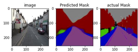
Pretty nice, this seems our auto-encoder worked well for this problem, but wait don’t you feel the results obtained are a bit fuzzy, what might have gone wrong?
Now the reason behind this fuzziness is there is a loss in feature map taking place when the information is passed from the encoder to the decoder as a result of this even though we can accomplish our goal the quality of output is just not good enough. So the most logical approach would be to connect the decoder layers with their counterparts in the encoder layers hence compensating for the features lost while reconstructing the image, that is what architectures like U-Net do. This can be better understood from the following figure:
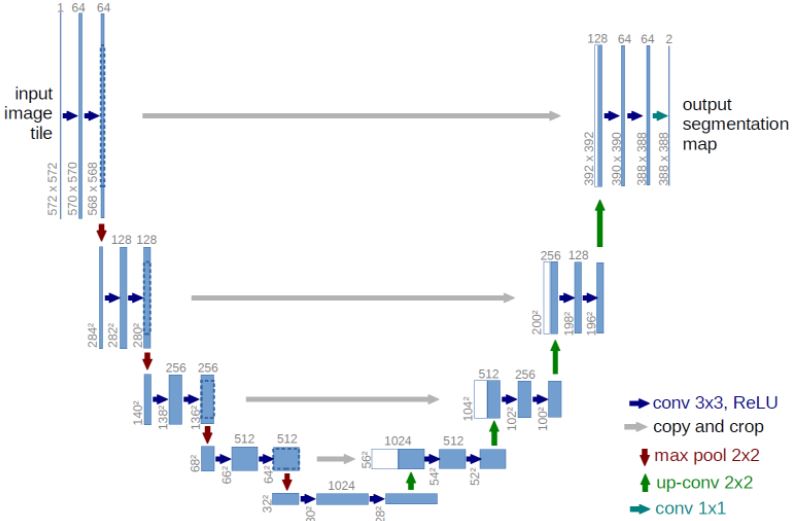
Have a look at the interconnection between the decoder and encoder layers, these make architectures like U-Net superior over vanilla auto-encoders. With this being said let’s discuss a few more practical applications that you can build using UNet.
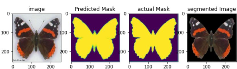
Here’s another segmentation problem for you that is different from the above-mentioned example. Given an image, you will be asked to predict a binary mask for the object of interest in the image, when you multiply this predicted mask and given image you will get the object of interest. Such prediction models can be used to find the location of the cancer cells or stones in the kidney. Since the worth of an image is more than a thousand words, here’s an image that shows what I am talking about:
Here is the code defining the architecture of the model used.
# defining Conv2d block for our u-net
# this block essentially performs 2 convolution
def Conv2dBlock(inputTensor, numFilters, kernelSize = 3, doBatchNorm = True):
    #first Conv
    x = tf.keras.layers.Conv2D(filters = numFilters, kernel_size = (kernelSize, kernelSize),
                              kernel_initializer = 'he_normal', padding = 'same') (inputTensor)
    if doBatchNorm:
        x = tf.keras.layers.BatchNormalization()(x)
    x =tf.keras.layers.Activation('relu')(x)
    #Second Conv
    x = tf.keras.layers.Conv2D(filters = numFilters, kernel_size = (kernelSize, kernelSize),
                              kernel_initializer = 'he_normal', padding = 'same') (x)
    if doBatchNorm:
        x = tf.keras.layers.BatchNormalization()(x)
    x = tf.keras.layers.Activation('relu')(x)
    return x

# Now defining Unet
def GiveMeUnet(inputImage, numFilters = 16, droupouts = 0.1, doBatchNorm = True):
    # defining encoder Path
    c1 = Conv2dBlock(inputImage, numFilters * 1, kernelSize = 3, doBatchNorm = doBatchNorm)
    p1 = tf.keras.layers.MaxPooling2D((2,2))(c1)
    p1 = tf.keras.layers.Dropout(droupouts)(p1)
    c2 = Conv2dBlock(p1, numFilters * 2, kernelSize = 3, doBatchNorm = doBatchNorm)
    p2 = tf.keras.layers.MaxPooling2D((2,2))(c2)
    p2 = tf.keras.layers.Dropout(droupouts)(p2)
    c3 = Conv2dBlock(p2, numFilters * 4, kernelSize = 3, doBatchNorm = doBatchNorm)
    p3 = tf.keras.layers.MaxPooling2D((2,2))(c3)
    p3 = tf.keras.layers.Dropout(droupouts)(p3)
    c4 = Conv2dBlock(p3, numFilters * 8, kernelSize = 3, doBatchNorm = doBatchNorm)
    p4 = tf.keras.layers.MaxPooling2D((2,2))(c4)
    p4 = tf.keras.layers.Dropout(droupouts)(p4)
    c5 = Conv2dBlock(p4, numFilters * 16, kernelSize = 3, doBatchNorm = doBatchNorm)
    # defining decoder path
    u6 = tf.keras.layers.Conv2DTranspose(numFilters*8, (3, 3), strides = (2, 2), padding = 'same')(c5)
    u6 = tf.keras.layers.concatenate([u6, c4])
    u6 = tf.keras.layers.Dropout(droupouts)(u6)
    c6 = Conv2dBlock(u6, numFilters * 8, kernelSize = 3, doBatchNorm = doBatchNorm)
    u7 = tf.keras.layers.Conv2DTranspose(numFilters*4, (3, 3), strides = (2, 2), padding = 'same')(c6)
    u7 = tf.keras.layers.concatenate([u7, c3])
    u7 = tf.keras.layers.Dropout(droupouts)(u7)
    c7 = Conv2dBlock(u7, numFilters * 4, kernelSize = 3, doBatchNorm = doBatchNorm)
    u8 = tf.keras.layers.Conv2DTranspose(numFilters*2, (3, 3), strides = (2, 2), padding = 'same')(c7)
    u8 = tf.keras.layers.concatenate([u8, c2])
    u8 = tf.keras.layers.Dropout(droupouts)(u8)
    c8 = Conv2dBlock(u8, numFilters * 2, kernelSize = 3, doBatchNorm = doBatchNorm)
    u9 = tf.keras.layers.Conv2DTranspose(numFilters*1, (3, 3), strides = (2, 2), padding = 'same')(c8)
    u9 = tf.keras.layers.concatenate([u9, c1])
    u9 = tf.keras.layers.Dropout(droupouts)(u9)
    c9 = Conv2dBlock(u9, numFilters * 1, kernelSize = 3, doBatchNorm = doBatchNorm)
    output = tf.keras.layers.Conv2D(1, (1, 1), activation = 'sigmoid')(c9)
    model = tf.keras.Model(inputs = [inputImage], outputs = [output])
    return model
Kindly refer to the references section of this article for the entire training pipeline.
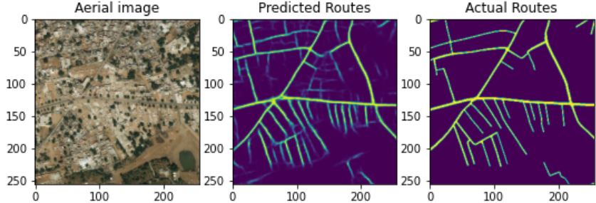
You can apply the above-mentioned architecture for finding roads in satellite images because if you think of this, it’s again a segmentation problem, with a proper data set you can easily achieve this task. As always here is an image showing this concept.
As always you can find the code in References Section.
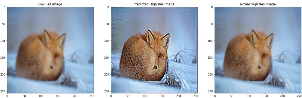
Have you ever noticed while zooming in on a low-resolution image, the pixel distortion that takes place? Super – Resolution essentially means to increase the resolution of a low-resolution image. Now, this can also be achieved just by upsampling the image and using bilinear interpolation to fill in the new pixel values, but then so the image generated will be blurry as you cannot increase the amount of information in the image. To combat this problem we teach a neural network to predict the pixel values for the high-resolution image (essentially adding information). You can achieve this using autoencoder (that’s the reason why the title of this article says “Endless world of Possibilities” !). You just have to make a small change in the above architecture just by changing the number of channels to 3 instead of 1 in the output layer of the model. Here a few results:
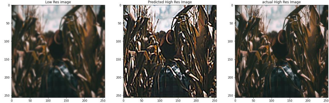
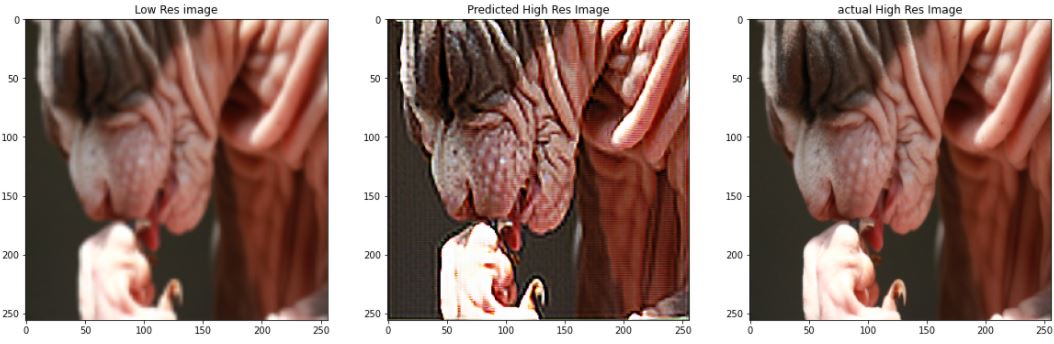
check the references section for the code and training pipeline.
These are just a few applications that I managed to build using auto-encoders but the possibilities are endless, and hence I would recommend the reader to let her/his creativity run wild and find even better uses for auto-encoders. Thanks.
CNN autoencoders are a type of neural network that uses CNNs to learn a compressed representation of its input data. They are typically used for unsupervised learning tasks, such as image denoising, inpainting, compression, and anomaly detection.
Autoencoders are a type of neural network that can be used to improve image quality, inpaint images, and detect anomalous images. They are being used in a variety of applications, such as medical imaging, remote sensing, and security.
2.) UNet Code and Binary Segmentation
3.) UNet for Road map generation from aerial Images.
4.) Super Resolution
The media shown in this article are not owned by Analytics Vidhya and is used at the Author’s discretion.
Lorem ipsum dolor sit amet, consectetur adipiscing elit,


