Probability distributions are fundamental tools in statistics and data science, providing a way to model and understand the uncertainty in various phenomena. Discrete probability distributions, such as the binomial and Poisson distributions, deal with outcomes that can be counted and are often used to analyze discrete random variables. These distributions are essential for predicting and understanding outcomes ranging from the number of successes in a fixed number of trials to the number of customers visiting a store in a day. Let’s explore the fascinating world of discrete probability distributions and their applications in modeling and predicting random events.
Learning Outcomes
- Understand the concept of expected value in the context of discrete probability distributions, where it represents the long-term average value of outcomes based on their probabilities.
- Learn how the sum of probabilities of all possible outcomes in a discrete probability distribution always equals 1, ensuring that one of the outcomes must occur.
- Recognize the fair coin as an example of a Bernoulli trial in probability theory, where the probability of heads and tails are both 0.5.
- Understand the concept of a fair dice, which has 6 equally probable outcomes (1 through 6) in a uniform distribution.
- Gain insight into uniform distribution, which describes a set of outcomes where each has an equal probability of occurring, such as rolling a fair dice.
This article was published as a part of the Data Science Blogathon.
Table of contents
What is Discrete Probability Distributions?
Discrete probability distributions represent the likelihood of different outcomes in a discrete set, such as the results of rolling a dice or the number of successes in a fixed number of trials. Each outcome is associated with a probability, and when graphed, these probabilities create a distribution. Common examples include the binomial distribution for binary events and the Poisson distribution for rare events. Such distributions are essential in statistics and probability theory for modeling and analyzing discrete random variables.
Discrete probability distributions are graphs of the outcomes of test results, such as a value of 1, 2, 3, true, false, success, or failure. Investors use discrete probability distributions to estimate the chances that a particular investing outcome is more or less likely to happen.
Understanding Discrete Probability Distributions with an Example
Let X be a random variable that has more than one possible outcome. Plot the probability on the y-axis and the outcome on the x-axis. If we repeat the experiment many times and plot the probability of each possible outcome, we get a plot that represents the probabilities. This plot is called the probability distribution (PD). The height of the graph for X gives the probability of that outcome.

Types of Probability Distributions
There are two types of distributions based on the type of data generated by the experiments.
1. Discrete Probability Distributions
These distributions model the probabilities of random variables that can have discrete values as outcomes. For example, the possible values for the random variable X that represents the number of heads that can occur when a coin is tossed twice are the set {0, 1, 2} and not any value from 0 to 2 like 0.1 or 1.6.
Examples: Bernoulli, Binomial, Negative Binomial, Hypergeometric, etc.,
2. Continuous Probability Distributions
These distributions model the probabilities of random variables that can have any possible outcome. For example, the possible values for the random variable X that represents weights of citizens in a town which can have any value like 34.5, 47.7, etc.,
Examples: Normal, Student’s T, Chi-square, Exponential, etc.,
Also Read: Basics of Probability for Data Science explained with examples in R
Terminologies
Each PD provides us extra information on the behavior of the data involved. Each PD is given by a probability function that generalizes the probabilities of the outcomes.
Using this, we can estimate the probability of a particular outcome(discrete) or the chance that it lies within a particular range of values for any given outcome(continuous). The function is called a Probability Mass function (PMF) for discrete distributions and a Probability Density function (PDF) for continuous distributions. The total value of PMF and PDF over the entire domain is always equal to one.
Cumulative Distribution Function
The PDF gives the probability of a particular outcome whereas the Cumulative Distribution Function gives the probability of seeing an outcome less than or equal to a particular value of the random variable. CDFs are used to check how the probability has added up to a certain point. For example, if P(X = 5) is the probability that the number of heads on flipping a coin is 5 then, P(X <= 5) denotes the cumulative probability of obtaining 1 to 5 heads.
Cumulative distribution functions are also used to calculate p-values as a part of performing hypothesis testing.
Discrete Probability Distributions
There are many discrete probability distributions to be used in different scenarios. We will discuss Discrete distributions in this post. Binomial and Poisson distributions are the most discussed ones in the following list.
- Bernoulli Distribution
- Binomial Distribution
- Hypergeometric Distribution
- Negative Binomial Distribution
- Geometric Distribution
- Poisson Distribution
- Multinomial Distribution
Types of Discrete Probability Distributions
Here are the list of types of Discrete probability distributions explained with examples.
Bernoulli Distribution
This distribution is generated when we perform an experiment once and it has only two possible outcomes – success and failure. The trials of this type are called Bernoulli trials, which form the basis for many distributions discussed below. Let p be the probability of success and 1 – p is the probability of failure.
The PMF is given as
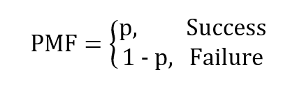
One example of this would be flipping a coin once. p is the probability of getting ahead and 1 – p is the probability of getting a tail. Please note down that success and failure are subjective and are defined by us depending on the context.
Binomial Distribution
This is generated for random variables with only two possible outcomes. Let p denote the probability of an event is a success which implies 1 – p is the probability of the event being a failure. Performing the experiment repeatedly and plotting the probability each time gives us the Binomial distribution.
The most common example given for Binomial distribution is that of flipping a coin n number of times and calculating the probabilities of getting a particular number of heads. More real-world examples include the number of successful sales calls for a company or whether a drug works for a disease or not.
The PMF is given as,
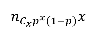
where p is the probability of success, n is the number of trials and x is the number of times we obtain a success.
Hypergeometric Distribution
Consider an event of drawing a red marble from a box of marbles with different colors. The event of drawing a red ball is a success and not drawing it is a failure. But each time a marble is drawn it is not returned to the box and hence this affects the probability of drawing a ball in the next trial. The hypergeometric distribution models the probability of k successes over n trials where each trial is conducted without replacement. This is unlike the binomial distribution where the probability remains constant through the trials.
The PMF is given as,
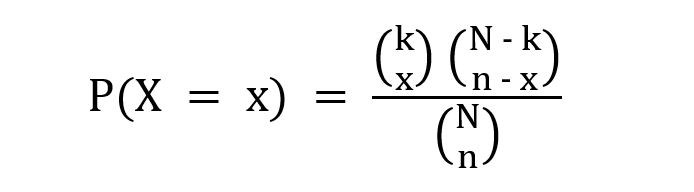
where k is the number of possible successes, x is the desired number of successes, N is the size of the population and n is the number of trials.
Negative Binomial Distribution
Sometimes we want to check how many Bernoulli trials we need to make in order to get a particular outcome. The desired outcome is specified in advance and we continue the experiment until it is achieved. Let us consider the example of rolling a dice. Our desired outcome, defined as a success, is rolling a 4. We want to know the probability of getting this outcome thrice. This is interpreted as the number of failures (other numbers apart from 4) that will occur before we see the third success.
The PMF is given as,
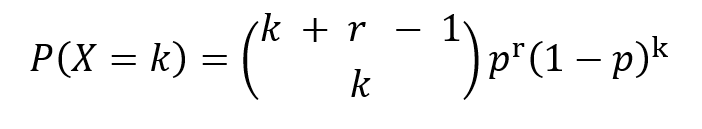
p indicates success probability, k is failures observed, and r specifies desired successes.
Like in Binomial distribution, the probability through the trials remains constant and each trial is independent of the other.
Geometric Distribution
This is a special case of the negative binomial distribution where the desired number of successes is 1. It measures the number of failures we get before one success. Using the same example given in the previous section, we would like to know the number of failures we see before we get the first 4 on rolling the dice.
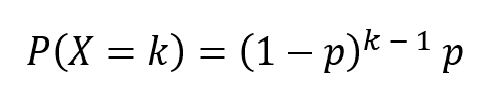
where p is the probability of success and k is the number of failures. Here, r = 1.
Poisson Distribution
This distribution describes the events that occur in a fixed interval of time or space. An example might make this clear. Consider the case of the number of calls received by a customer care center per hour. We can estimate the average number of calls per hour but we cannot determine the exact number and the exact time at which there is a call. Each occurrence of an event is independent of the other occurrences.
The PMF is given as,
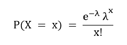
where λ is the average number of times the event has occurred in a certain period of time, x is the desired outcome and e is the Euler’s number.
Multinomial Distribution
In the above distributions, there are only two possible outcomes – success and failure. The multinomial distribution, however, describes the random variables with many possible outcomes. This is also sometimes referred to as categorical distribution because it treats each possible outcome as a separate category. Consider the scenario of playing a game n number of times. Multinomial distribution calculates the combined probability of player wins across multiple trials.
The PMF is given as,
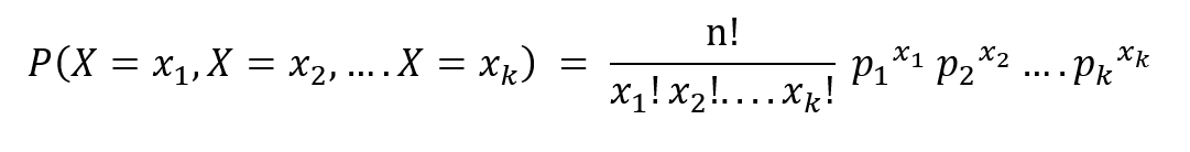
where n is the number of trials, p1,……pk denote the probabilities of the outcomes x1……xk respectively.
Discrete vs Continuous Distribution
| Discrete Distribution | Continuous Distribution |
|---|---|
| Random variable can only take on a finite or countable number of values | Random variable can take on any value within a certain range or interval |
| Probability function assigns probabilities to each possible outcome | Probability function assigns probabilities to each possible value within a range or interval |
| Examples: binomial distribution, Poisson distribution, geometric distribution | Examples: normal distribution, exponential distribution, beta distribution |
| Used to model events with discrete outcomes, such as number of successes in a fixed number of trials | Used to model events with continuous outcomes, such as the height of individuals in a population |
| Probability of any single outcome is non-zero | Probability of any single value is zero |
| Cumulative distribution function is stepwise | Cumulative distribution function is continuous |
Also Read: Understanding Random Variables their Distributions
Conclusion
Discrete probability distributions are essential tools for modeling and predicting outcomes of random events with discrete results, such as the number of customers visiting a store or the outcomes of coin tosses and dice rolls. This article has explored several key types of discrete probability distributions, including Bernoulli, Binomial, Hypergeometric, Negative Binomial, Geometric, Poisson, and Multinomial distributions, each suited for different scenarios in probability theory.
This article discusses concepts such as expected value, the sum of probabilities, fair coin experiments, fair dice outcomes, and uniform distribution to provide a comprehensive understanding. Mastering these foundational concepts is crucial as they enable informed decisions and predictions based on statistical data. This enhances data-driven decision-making capabilities across various fields, ensuring accurate analysis and interpretation of outcomes.
Frequently Asked Questions
Q1. What is discrete and continuous distribution?
A. Discrete distributions are probability distributions where a random variable can only take on finite or countable values. Continuous distributions allow the random variable to take on any value within a certain range.
Q2. What is the difference between discrete variables and continuous random variables?
A. Discrete variables are integers within a sample space, like the number of heads in a coin flip or event occurrences. Continuous random variables, like height, weight, or temperature, can take any numerical value within a range or interval, with probabilities defined over an interval.
Q3. How is a histogram used in understanding a probability distribution function?
A. A histogram is a visual representation of a dataset, used to estimate the probability distribution function of discrete and continuous random variables. It visualizes the frequency of data points within consecutive intervals, providing a visual representation of the data’s distribution, standard deviation, and central tendency.
Q4. What parameters define a binomial probability distribution, and how is the standard deviation calculated?
A. A binomial probability distribution is a statistical model that considers the number of trials and the probability of success on each trial. It is based on the fact that trials are independent and only two outcomes are possible. The standard deviation, calculated using a formula, measures the variation in actual outcomes from the expected number of successes.
The media shown in this article are not owned by Analytics Vidhya and is used at the Author’s discretion.
Priyanka Madiraju
27 May, 2024


