Understanding Random Variable in Statistics

Introduction

Why should we care about random variables and their distributions? Let’s explore this important concept in statistics. We’ll break down the basics of probability, understand what random variables are, and see why their distributions matter. Whether you’re new to this or want a refresher, this guide is here to help you grasp these essential ideas and feel more comfortable with statistics. In this article you Will get to know about the Random Variables in Statistics and also definition of random variable, so basically this article is a complete guide for Random Variables.

This article was published as a part of the Data Science Blogathon.

What are Random Variables?

A random variable, also known as a stochastic variable, functions in the realm of real values within the entire sample space of an experiment. Imagine the domain as the pool of all possible values applicable to the function. Just as a function processes its domain, a random variable operates on its domain (the experiment’s sample space) and assigns a real value to each event or outcome.

The collection of these real values, derived from the random variable, forms its range. In statistical notation, a random variable is typically denoted by a capital letter, while its observed values go by small letters.

Consider the experiment of tossing two coins. We can define X to be a random variable that measures the number of heads observed in the experiment. The sample set is here:

There are 4 possible outcomes for the experiment, and this is the domain of X. The random variable X takes these 4 outcomes/events and processes them to give different real values. For each outcome, the associated value is shown as:

Thus, we can represent X as follows:

Also Read: End to End Statistics for Data Science

Types of Random Variables

There are three types of random variables- discrete random variables, continuous random variables, and mixed random variables.

Discrete Random Variables

Discrete random variables are random variables, whose range is a countable set. A countable set can be either a finite set or a countably infinite set. For instance, in the above example, X is a discrete variable as its range is a finite set ({0, 1, 2}).

Continuous Random Variables

Continuous random variables, on the contrary, have a range in the forms of some interval, bounded or unbounded, of the real line. E.g., Let Y be a random variable that is equal to the height of different people in a given population set. Since the people can have different measures of height (not limited to just natural numbers or any countable set), Y is a continuous variable (in fact, the distribution of Y follows a normal/gaussian distribution on most occasions).

Mixed Random Variables

Lastly, mixed random variables are ones that are a mixture of both continuous and discrete variables. These variables are more complicated than the other two. Hence, they are explained at the end of this article.

What is Random Variables in Statisitics?

In statistics, a random variable is essentially a numeric portrayal of the result of an experimental event involving uncertainty. It functions as an interpreter which converts the arbitrary outcomes into numerical data that can be examined using mathematics.

Here is an overview of the main highlights:

Giving Numbers to Results: Picture tossing a coin. We can either get heads or tails as outcomes, which we can represent statistically by assigning the number 1 to heads and 0 to tails. This rule assignment is a random variable.

Two Varieties: Discrete vs Continuous: Random variables fall into two primary categories:

Discreet: These variables only assume distinct, separate values. Similar to the number of times a coin lands heads in ten flips (0, 1, 2, …, 10).

Ongoing: These variables have the ability to have any value in a specified range. For instance, the scale measures the weight of a person within a specific range of values.

Probability Distribution of Random Variables

When we express the likelihood of values in a random variable’s range, we essentially discuss the probability distribution of that random variable. This means calculating the probability for each value within the variable’s range. Probability distribution descriptions differ slightly for discrete and continuous random variables.

The Discrete Case

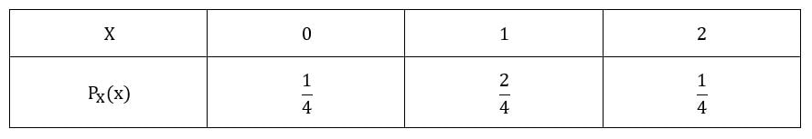
For discrete variables, the term ‘Probability mass function (PMF)’ is used to describe their distributions. Using the example of coin tosses, as discussed above, we calculate the probability of X taking the values 0, 1 and 2 as follows:

We use the notation P_X(x) to refer to
the PMF of the random variable X. The distribution is shown as follows:

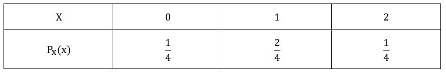
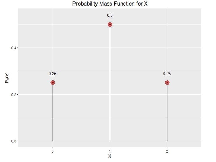
The table can also be graphically demonstrated:

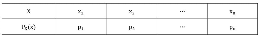
In general, if a random variable X has a countable range given by:

Then, we define probability mass function as:

This also leads us to the general description of the distribution in tabular format:

Properties of probability mass function:

1) PMF can never be more than 1 or negative i.e.,

2) PMF must sum to one over the entire range set of a random variable.

3) For A, a subset of R_x,

The Continuous Case

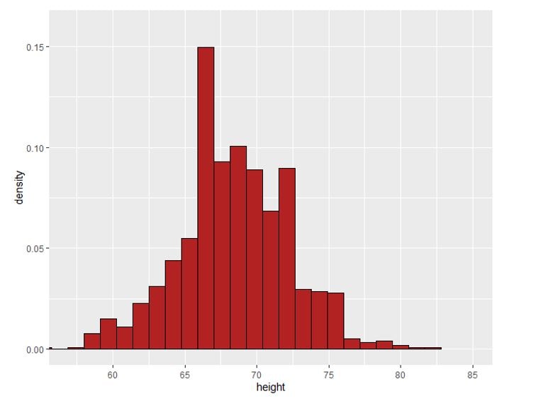
For continuous variables, the term ‘Probability density function (PDF)’ is used to describe their distributions. We’ll consider the example of the distribution of heights. Suppose, we survey a group of 1000 people and measure the height of each person very precisely. The distribution of the heights can be shown by a density histogram as follows:

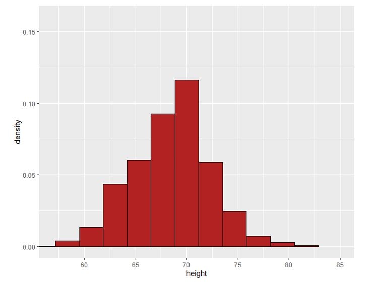
We have grouped the different heights in certain intervals. But let’s see what happens when we try to reduce the size of the histogram bins. In other words, we make the grouping intervals smaller and smaller.

Going further, we further reduce the bin size to such an extent that every observation tends to have its own bin. We are essentially constructing these extremely tiny rectangles, that we connect together by a smooth curve, giving us the following distribution:

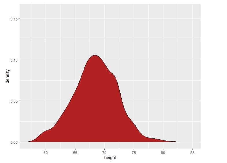
And that’s it! We have got the probability distribution of heights for our sample population set. But how’s probability related to all of this? Observe the y axis. It shows density, which indicates the proportion of the population having a particular range of height. The probability that a randomly chosen person from the population having a height within the given interval corresponds to this proportion. That sounds more probabilistic!

We use the notation f_X(x) to refer to the PDF of random variable X. Both PMF and PDF are analogous. We just replace summation with integration to account for their continuous behaviour.

Properties of Probability Density Function

1) PDF can never negative i.e.,

2) PDF must integrate to one over the entire range of a random variable.

3) For A, a subset of R_x,

More specifically, if A = [a, b], then,

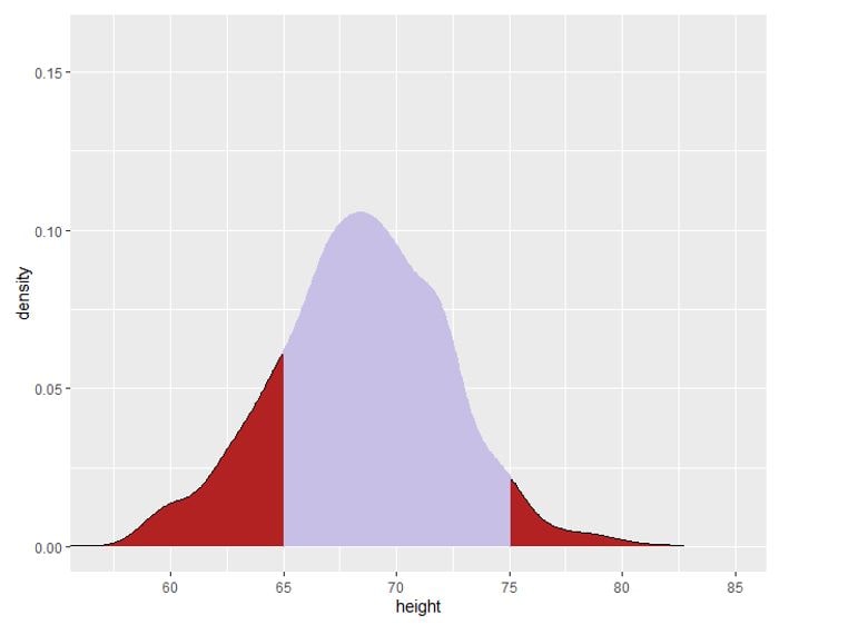
Graphically, the probability that a continuous random variable X takes a value within a given interval is the area below the PDF for X, enclosed between the given interval. For instance, in the above example, if we wish to determine the probability that a randomly selected person from the population has a height between 65 cm and 75 cm, we calculate the purple area (using definite integration):

Note: Unlike PMF, PDF can take a value greater than 1. This is because of a difference in their interpretation. In the case of PMF, the value of the function for a particular x has the same interpretation as probability, making its value restricted to the [0, 1] interval. However, in PDF, the value does not translate to probability. In fact, P(X = x) = 0, if X is a continuous variable (it’s like calculating area under the PDF curve, just below a point).

Cumulative Distribution of Random Variables

Sometimes, it’s easier to have the distribution of a random variable expressed in an alternative way. Cumulative distribution functions (CDF) are one such way. Cumulate means to gather or sum up. CDFs do the same. A useful property of CDFs is that they are defined in the same way for both discrete and continuous variables. A CDF shows the probability that a random variable X takes a value lesser than or equal to x. Mathematically, a CDF is defined as follows:

Let’s consider both the discrete and the continuous case.

The Discrete Case

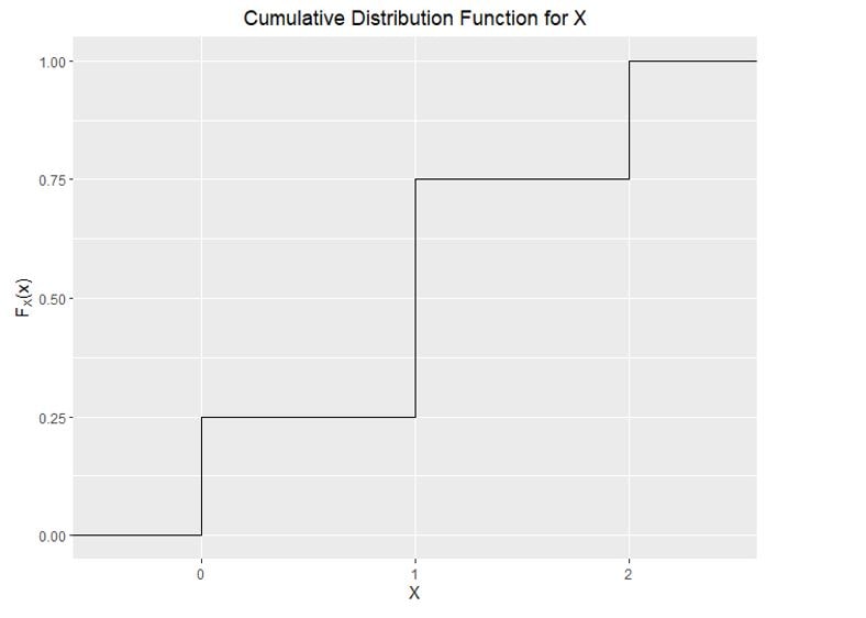
The CDF of discrete random variables resembles a staircase, a graph with many jumps. We’ll again use the coin toss example. The following PMF was obtained:

We’ll now calculate the CDF of X for different values of x:

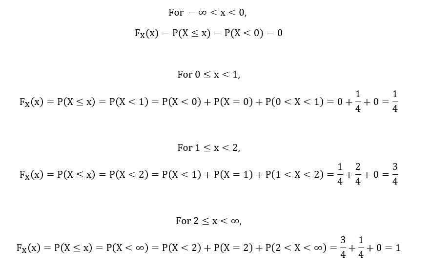
Hence, we can define F_X(x) as follows:

The CDF can also be shown graphically as follows:

For discrete variables, we can define the following relation between PMF and CDF:

The Continuous Case

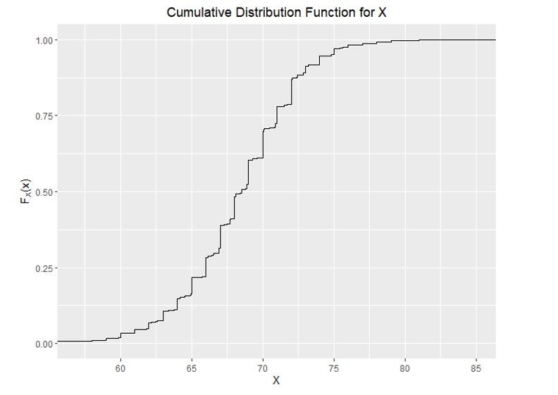
The CDF of continuous random variables is noisier than that of discrete variables. Just as previously done, we sum up (rather say, integrate) the PDF to get the CDF. For the example of the height, the following CDF has been made:

For continuous variables, we can define the following relation between PDF and CDF:

Properties of CDF

1) CDF is always a non-decreasing function.

2) CDF always lies between 0 and 1.

3) For all a < b,

Expectation & Variance of Random Variables

Many times, it’s handy to use just a few numbers to express the distribution of a random variable. There are many such numbers- most common of which are expectation and variance.

The Expectation of Random Variables

The expectation (also known as mean) of a random variable X is its weighted average. For discrete random variables, the expectation is calculated using the following equation:

For continuous variables, once again, we replace summation with integration to arrive at the following equation:

Basic properties of expectation of random variables:

1) The expectation of a constant is the constant itself.

2) The expectation of the sum of two random variables is equal to the sum of their expectations.

3) If Y = aX + b, then the expectation of Y is calculated as:

The Variance of Random Variables

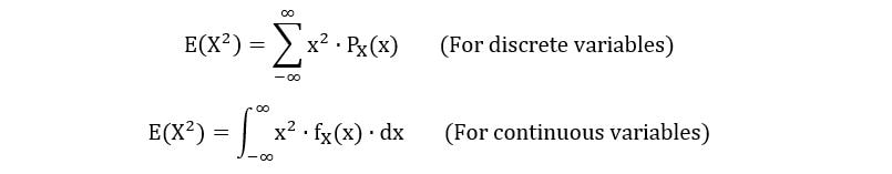
The variance of a random variable X is the expected value of the square of the deviation of different values of X from the expectation of X. It shows the spread of the distribution of a random variable is. It is generally represented as:

However, a more useful expression for variance is obtained after simplifying the above equation:

Where,

Basic properties of variance of random variables:

1) The variance of a constant is zero.

2) For two random variables- X & Y, the variance of their sum is expressed as follows:

Cov(X, Y) is called the covariance of X & Y. Covariance describes the relationship between two variables. It can be defined by the following equation:

3) If Y = aX + b, then the variance of Y is defined as:

Mixed Random Variables

Mixed random variables have a discrete part (where the range of the variable is a countable set), and a continuous part (where the range of the variable takes the form of an interval of the real line). A mixed random variable Z can be shown as follows:

The CDF of the mixed random variable Z can be found out by calculating the weighted average of its components:

The expectation of Z can also be calculated by using the above methodology:

Conclusion

In conclusion, understanding random variables and their distributions is fundamental to unraveling the mysteries of probability and statistics. We’ve taken a journey through the basics, delving into the significance of these concepts. Whether navigating data analysis, research, or simply enhancing your statistical literacy, a solid grasp of random variables and distributions empowers you to interpret, analyze, and draw meaningful insights from a world of uncertainty. Embrace the power of probability, and let these concepts guide you in making sense of the randomness surrounding us.

Hope you like the article and getting understanding of random variables in statistics and from the definition of random variable to random variable in probability you get the full understanding.

Frequently Asked Questions

The media shown in this article are not owned by Analytics Vidhya and is used at the Author’s discretion.