Seismic Analysis with Python

This article was published as a part of the Data Science Blogathon.

In this article, we will try to study the relationship between worldwide earthquake distributions and tectonic plate boundaries. Earthquakes are one of the major Natural Disasters which killed around 750,000 people worldwide from 1998 to 2017( Source: World Health Organization ). the worst one India ever had to face was the Indian Ocean Earthquake which took place in December 26, 2004. I personally have a connection to this earthquake. I’ve spent my childhood in numerous states, and during that time, just after a few months from the earthquake and the resulting tsunami, we were headed for Andaman and Nicobar Islands, where we’d spend the next 4 years.

Seeing the effects of that devastating Tsunami firsthand had been quite an experience for my childhood self.

India ocean Earthquake, 2004

Date: December 26, 2004

Time: 08:50

Deaths: 283,106

Affected countries: Indonesia, Sri Lanka, India, Thailand, Maldives, and Somalia.

Seismic Analysis

For this analysis we will use 2 datasets from Kaggle, which are:

Significant Earthquakes, 1965-2016

Tectonic Plate Boundaries

Most of the origins of Earthquakes can be traced back to geological causes, namely the dynamics of tectonic plates. However, some other reasons can be Volcanic inflation, explosions, Deep penetration bombs, Climate change, etc.

1) Importing Libraries

# Importing Libraries
import numpy as np
import pandas as pd
import geopandas as gpd
import matplotlib.pyplot as plt
import seaborn as sns
import folium
from folium import Choropleth
from folium.plugins import HeatMap
import datetime

np.<a onclick="parent.postMessage({'referent':'.numpy.random'}, '*')">random.seed(0)

2) Loading Data

Python Code:

# Importing Libraries
import numpy as np
import pandas as pd
import geopandas as gpd
import matplotlib.pyplot as plt
import seaborn as sns
import folium
from folium import Choropleth
from folium.plugins import HeatMap
import datetime

np.random.seed(0)

#loading data
#eathquake data
data = pd.read_csv('database.csv')
#dropping columns with missing values
missing_values_columns = [col for col in data.columns if data[col].isnull().any()]
data = data.drop(missing_values_columns, axis=1)
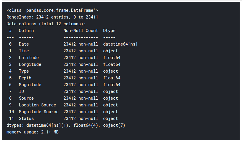
print(data.head())

##Resize the size of the window .Scroll right to the see the data head in the output window

Loading data for tectonic plate boundaries

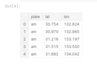
#loading data for tectonic plate boundaries
tectonic_plates = pd.<a onclick="parent.postMessage({'referent':'.pandas.read_csv'}, '*')">read_csv("../input/tectonic-plate-boundaries/all.csv" )
tectonic_plates.head()

2) Data Preprocessing

Steps to preprocess the data

• Date parsing: Parsing date to dtype datetime64(ns)
• Time Parsing: Parsing time to dtype timedelta64
• Adding Attributes: ” Date_Time ” and ” Days “

#Parsing datetime
#exploring the length of date objects
lengths = data["Date"].str.len()
lengths.value_counts()

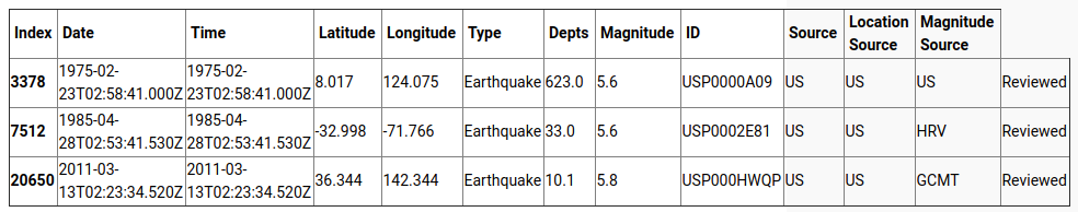
#having a look at the fishy datapoints
wrongdates = np.<a onclick="parent.postMessage({'referent':'.numpy.where'}, '*')">where([lengths == 24])[1]
print("Fishy dates:", wrongdates)
data.loc[wrongdates]

#fixing the wrong dates and changing the datatype from numpy object to datetime64[ns]
data.loc[3378, "Date"] = "02/23/1975"  
data.loc[7512, "Date"] = "04/28/1985"
data.loc[20650, "Date"] = "03/13/2011"
data['Date']= pd.<a onclick="parent.postMessage({'referent':'.pandas.to_datetime'}, '*')">to_datetime(data["Date"])
data.info()

#We have time data too. Now that we are at it,lets parse it as well. 
#exploring the length of time objects
lengths = data["Time"].str.len()
lengths.value_counts()

#Having a look at the fishy datapoints
wrongtime = np.where([lengths == 24])[1]
print("Fishy time:", wrongtime)
data.loc[wrongtime]

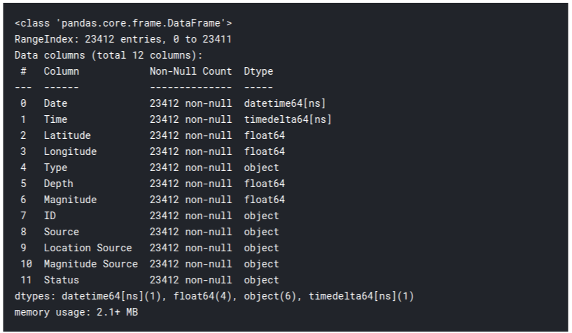
#Ah! Is it deja vu or are those the same datapoints
#fixing the wrong time and changing the datatype from numpy object to timedelta64[ns]
data.loc[3378, "Time"] = "02:58:41"
data.loc[7512, "Time"] = "02:53:41"
data.loc[20650, "Time"] = "02:23:34"
data['Time']= pd.<a onclick="parent.postMessage({'referent':'.pandas.to_timedelta'}, '*')">to_timedelta(data['Time'])
data.info()

#I don't think there is any point in doing this step, but why not!
data["Date_Time"]=data["Date"] +data["Time"]

#Now that we have Date, Time (and Date_Time) we totally should have Days of week too.
data["Days"]= data.Date.dt.strftime("%A")

#Lets have a look at data
data.head()

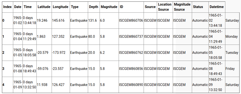
( Note: The last column is named “Days”.)

3) Data Analysis

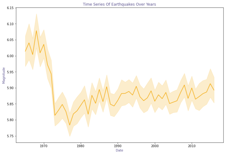
First, we make a line plot of magnitudes with dates. This will show a time series of various earthquakes around the world from 1965 to 2016. An initial inference that can be drawn by looking at the plot is that there was relatively high seismic activity from 1965 to the early 1970s.

#plotting a lineplot with magnitudes with respectto dates
plt.<a onclick="parent.postMessage({'referent':'.matplotlib.pyplot.figure'}, '*')">figure(figsize=(12,8))
Time_series=sns.<a onclick="parent.postMessage({'referent':'.seaborn.lineplot'}, '*')">lineplot(x=data['Date'].dt.year,y="Magnitude",data=data, color="#ffa600")
Time_series.set_title("Time Series Of Earthquakes Over Years", color="#58508d")
Time_series.set_ylabel("Magnitude", color="#58508d")
Time_series.set_xlabel("Date", color="#58508d")

However, our dataset contains earthquakes caused by other factors like normal explosions, Nuclear explosions, and rockburst. In order to draw a clear relation between seismic activities and earthquakes, we have to rule out the other factors.

#Plotting timeseries with respect to Type to geta better understanding
plt.<a onclick="parent.postMessage({'referent':'.matplotlib.pyplot.figure'}, '*')">figure(figsize=(12,8))
colours = ["#ffa600","#bc5090","#ff6361","#003f5c"]
Time_series_Type=sns.<a onclick="parent.postMessage({'referent':'.seaborn.lineplot'}, '*')">lineplot(x=data['Date'].dt.year,y="Magnitude",data=data,hue="Type", palette= colours)
Time_series_Type.set_title("Time Series Of Earthquakes Over Years (With Type)", color="#58508d")
Time_series_Type.set_ylabel("Magnitude", color="#58508d")
Time_series_Type.set_xlabel("Date", color="#58508d")

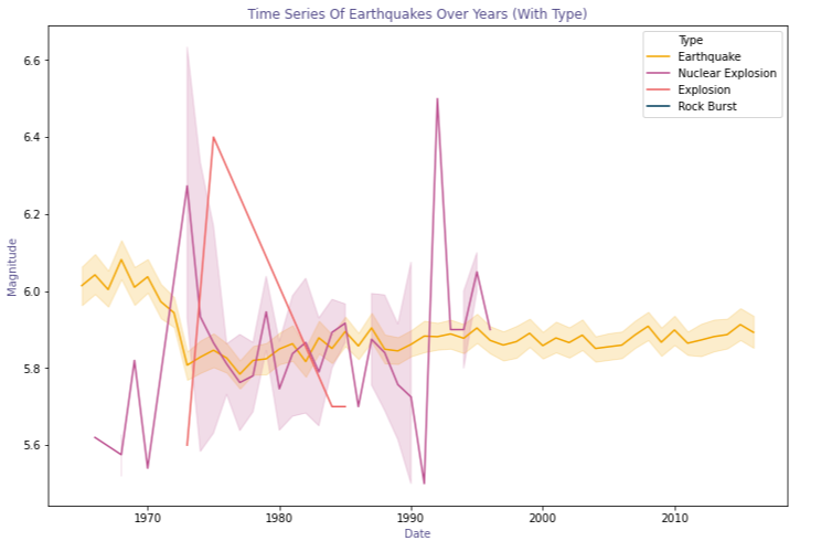
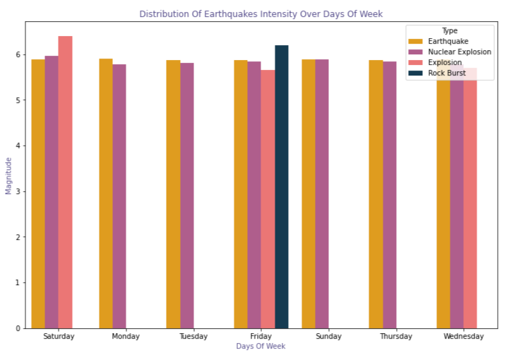
From the above plot, we can conclude that indeed the higher frequency of earthquakes is caused due to external reasons like nuclear explosions. In this next plot, we will see the distribution of quakes on the days of the week.

#Evauating earthquake in terms of days of week
plt.<a onclick="parent.postMessage({'referent':'.matplotlib.pyplot.figure'}, '*')">figure(figsize=(12,8))
Days_of_week=sns.<a onclick="parent.postMessage({'referent':'.seaborn.barplot'}, '*')">barplot(x=data['Days'],y="Magnitude",data=data, ci =None, hue ="Type",palette = colours)
Days_of_week.set_title("Distribution Of Earthquakes Intensity Over Days Of Week", color="#58508d")
Days_of_week.set_ylabel("Magnitude", color="#58508d")
Days_of_week.set_xlabel("Days Of Week", color="#58508d")

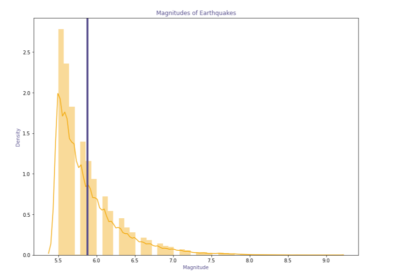
Now we plot the magnitude of earthquakes and mean magnitude.

#ploting the magnitude of earthquake and mean magnitute

plt.<a onclick="parent.postMessage({'referent':'.matplotlib.pyplot.figure'}, '*')">figure(figsize=(12,9))
strength = data["Magnitude"].values
mean_M= data["Magnitude"].mean()
Magnitude_plot = sns.<a onclick="parent.postMessage({'referent':'.seaborn.distplot'}, '*')">distplot(strength, color ="#ffa600")
Magnitude_plot.set_title("Magnitudes of Earthquakes", color="#58508d")
Magnitude_plot.set_ylabel("Density", color="#58508d")
Magnitude_plot.set_xlabel("Magnitude", color="#58508d")

plt.<a onclick="parent.postMessage({'referent':'.matplotlib.pyplot.axvline'}, '*')">axvline(mean_M,0,1, color="#58508d",linewidth=4,label="Mean")

Geospatial Analysis

Earth’s crust is divided into numerous segments called the tectonic plates. These plates are sometimes moved in little or huge amounts due to the geothermal energy generated in the Mantle of the Earth. These movements are mostly seen in the tectonic boundaries and are the major cause of natural Earthquakes.

In this section, we will try to find any correlation between earthquakes and the tectonic plates. First, we shall plot the tectonic boundaries on the map, and see if these boundaries hold any relation with the location of earthquakes.

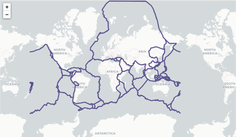
1) Tectonic plate boundaries plotted

#Ploting the tectonic plate's boundaries 
tectonic = folium.<a onclick="parent.postMessage({'referent':'.folium.Map'}, '*')">Map(tiles="cartodbpositron", zoom_start=5)

plates = list(tectonic_plates["plate"].unique())
for plate in plates:
    plate_vals = tectonic_plates[tectonic_plates["plate"] == plate]
    lats = plate_vals["lat"].values
    lons = plate_vals["lon"].values
    points = list(zip(lats, lons))
    indexes = [None] + [<a onclick="parent.postMessage({'referent':'.kaggle.usercode.13873697.58987243.[5527,5530].i'}, '*')">i + 1 for <a onclick="parent.postMessage({'referent':'.kaggle.usercode.13873697.58987243.[5527,5530].i'}, '*')">i, <a onclick="parent.postMessage({'referent':'.kaggle.usercode.13873697.58987243.[5527,5530].x'}, '*')">x in enumerate(points) if <a onclick="parent.postMessage({'referent':'.kaggle.usercode.13873697.58987243.[5527,5530].i'}, '*')">i < len(points) - 1 and abs(<a onclick="parent.postMessage({'referent':'.kaggle.usercode.13873697.58987243.[5527,5530].x'}, '*')">x[1] - points[<a onclick="parent.postMessage({'referent':'.kaggle.usercode.13873697.58987243.[5527,5530].i'}, '*')">i + 1][1]) > 300] + [None]
    for i in range(len(indexes) - 1):
        folium.<a onclick="parent.postMessage({'referent':'.folium.vector_layers'}, '*')">vector_layers.PolyLine(points[indexes[i]:indexes[i+1]], popup=plate, color="#58508d", fill=False, ).add_to(tectonic)

tectonic

2) Plate boundaries with natural earthquake locations

#plotting the the eartquake type to only earthquake

tectonic_quake = folium.<a onclick="parent.postMessage({'referent':'.folium.Map'}, '*')">Map(tiles="cartodbpositron", zoom_start=5)
plates = list(tectonic_plates["plate"].unique())
for plate in plates:
    plate_vals = tectonic_plates[tectonic_plates["plate"] == plate]
    lats = plate_vals["lat"].values
    lons = plate_vals["lon"].values
    points = list(zip(lats, lons))
    indexes = [None] + [<a onclick="parent.postMessage({'referent':'.kaggle.usercode.13873697.58987243.[7343,7346].i'}, '*')">i + 1 for <a onclick="parent.postMessage({'referent':'.kaggle.usercode.13873697.58987243.[7343,7346].i'}, '*')">i, <a onclick="parent.postMessage({'referent':'.kaggle.usercode.13873697.58987243.[7343,7346].x'}, '*')">x in enumerate(points) if <a onclick="parent.postMessage({'referent':'.kaggle.usercode.13873697.58987243.[7343,7346].i'}, '*')">i < len(points) - 1 and abs(<a onclick="parent.postMessage({'referent':'.kaggle.usercode.13873697.58987243.[7343,7346].x'}, '*')">x[1] - points[<a onclick="parent.postMessage({'referent':'.kaggle.usercode.13873697.58987243.[7343,7346].i'}, '*')">i + 1][1]) > 300] + [None]
    for i in range(len(indexes) - 1):
        folium.<a onclick="parent.postMessage({'referent':'.folium.vector_layers'}, '*')">vector_layers.PolyLine(points[indexes[i]:indexes[i+1]], popup=plate, fill=False,  color="#58508d").add_to(tectonic_quake)
        HeatMap(data=data_onlyquakes[["Latitude", "Longitude"]], min_opacity=0.5,max_zoom=40,max_val=0.5,radius=1,gradient=gradient).add_to(tectonic_quake)

tectonic_quake

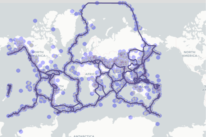
 We do not include all the occurrences of earthquakes because we just want the naturally occurring ones to correlate without tectonic plate boundaries. As you can see from the above map, a clear relationship between earthquakes and tectonic boundaries is found.

Now we shall access the magnitude and depths of these earthquakes. Let us go with magnitude first:

For the magnitudes, we will choose 3 ranges:

1. Less than 5.9
2. Less than 6.5
3. More than 6.5

# Create a base map with plate boundaries and depth 
Mag_tectonics  = folium.<a onclick="parent.postMessage({'referent':'.folium.Map'}, '*')">Map(tiles="cartodbpositron", zoom_start=5)
gradient = {.33: "#628d82", .66: "#a3c5bf", 1: "#eafffd"} 
plates = list(tectonic_plates["plate"].unique())
for plate in plates:
    plate_vals = tectonic_plates[tectonic_plates["plate"] == plate]
    lats = plate_vals["lat"].values
    lons = plate_vals["lon"].values
    points = list(zip(lats, lons))
    indexes = [None] + [<a onclick="parent.postMessage({'referent':'.kaggle.usercode.13873697.58987243.[8247,8250].i'}, '*')">i + 1 for <a onclick="parent.postMessage({'referent':'.kaggle.usercode.13873697.58987243.[8247,8250].i'}, '*')">i, <a onclick="parent.postMessage({'referent':'.kaggle.usercode.13873697.58987243.[8247,8250].x'}, '*')">x in enumerate(points) if <a onclick="parent.postMessage({'referent':'.kaggle.usercode.13873697.58987243.[8247,8250].i'}, '*')">i < len(points) - 1 and abs(<a onclick="parent.postMessage({'referent':'.kaggle.usercode.13873697.58987243.[8247,8250].x'}, '*')">x[1] - points[<a onclick="parent.postMessage({'referent':'.kaggle.usercode.13873697.58987243.[8247,8250].i'}, '*')">i + 1][1]) > 300] + [None]
    for i in range(len(indexes) - 1):
        folium.<a onclick="parent.postMessage({'referent':'.folium.vector_layers'}, '*')">vector_layers.PolyLine(points[indexes[i]:indexes[i+1]], fill=False,  color="#58508d").add_to(Mag_tectonics)
        
def colormag(<a onclick="parent.postMessage({'referent':'.kaggle.usercode.13873697.58987243.colormag..val'}, '*')">val):
            if <a onclick="parent.postMessage({'referent':'.kaggle.usercode.13873697.58987243.colormag..val'}, '*')">val < 5.9:
                return "#ffcf6a"
            elif <a onclick="parent.postMessage({'referent':'.kaggle.usercode.13873697.58987243.colormag..val'}, '*')">val < 6.5:
                return "#fb8270"
            else:
                return "#bc5090"
            
for i in range(0,len(data)):
    folium.<a onclick="parent.postMessage({'referent':'.folium.Circle'}, '*')">Circle(location=[data.iloc[i]["Latitude"], data.iloc[i]["Longitude"]],radius=2000, color=colormag(data.iloc[i]["Magnitude"])).add_to(Mag_tectonics)

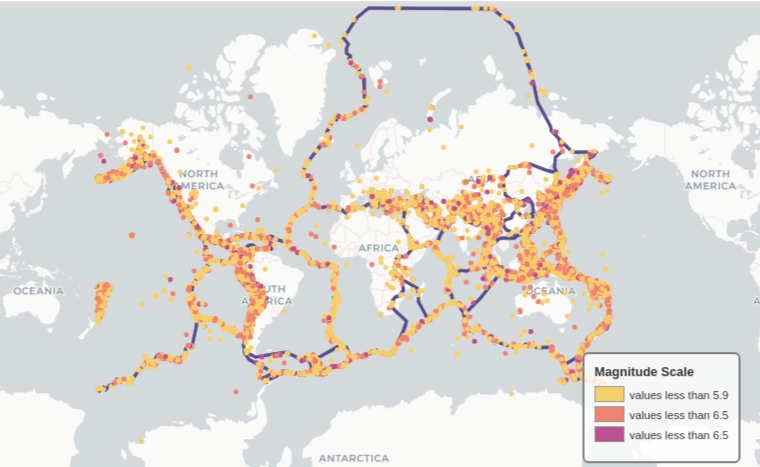
There is no clear relation between Magnitude distribution and plate boundaries. It seems to be randomly distributed. We can easily discard any hypothesis we might’ve had regarding the correlation of tectonic boundaries and earthquake location. Next is the Depth.

For Depth too, we shall choose 3 ranges:

1. Less than 50Km
2. Less than 100Km
3. More than 100Km

# Create a base map with plate boundaries and depth 
Depth_tectonics  = folium.<a onclick="parent.postMessage({'referent':'.folium.Map'}, '*')">Map(tiles="cartodbpositron", zoom_start=5)
gradient = {.33: "#628d82", .66: "#a3c5bf", 1: "#eafffd"} 
plates = list(tectonic_plates["plate"].unique())
for plate in plates:
    plate_vals = tectonic_plates[tectonic_plates["plate"] == plate]
    lats = plate_vals["lat"].values
    lons = plate_vals["lon"].values
    points = list(zip(lats, lons))
    indexes = [None] + [<a onclick="parent.postMessage({'referent':'.kaggle.usercode.13873697.58987243.[11483,11486].i'}, '*')">i + 1 for <a onclick="parent.postMessage({'referent':'.kaggle.usercode.13873697.58987243.[11483,11486].i'}, '*')">i, <a onclick="parent.postMessage({'referent':'.kaggle.usercode.13873697.58987243.[11483,11486].x'}, '*')">x in enumerate(points) if <a onclick="parent.postMessage({'referent':'.kaggle.usercode.13873697.58987243.[11483,11486].i'}, '*')">i < len(points) - 1 and abs(<a onclick="parent.postMessage({'referent':'.kaggle.usercode.13873697.58987243.[11483,11486].x'}, '*')">x[1] - points[<a onclick="parent.postMessage({'referent':'.kaggle.usercode.13873697.58987243.[11483,11486].i'}, '*')">i + 1][1]) > 300] + [None]
    for i in range(len(indexes) - 1):
        folium.<a onclick="parent.postMessage({'referent':'.folium.vector_layers'}, '*')">vector_layers.PolyLine(points[indexes[i]:indexes[i+1]],fill=False,  color="#58508d").add_to(Depth_tectonics)
        
def colordepth(<a onclick="parent.postMessage({'referent':'.kaggle.usercode.13873697.58987243.colordepth..val'}, '*')">val):
            if <a onclick="parent.postMessage({'referent':'.kaggle.usercode.13873697.58987243.colordepth..val'}, '*')">val < 50:
                return "#ffcf6a"
            elif <a onclick="parent.postMessage({'referent':'.kaggle.usercode.13873697.58987243.colordepth..val'}, '*')">val < 100:
                return "#fb8270"
            else:
                return "#bc5090"
            
for i in range(0,len(data)):
    folium.<a onclick="parent.postMessage({'referent':'.folium.Circle'}, '*')">Circle(location=[data.iloc[i]["Latitude"], data.iloc[i]["Longitude"]],radius=2000, color=colordepth(data.iloc[i]["Depth"])).add_to(Depth_tectonics)

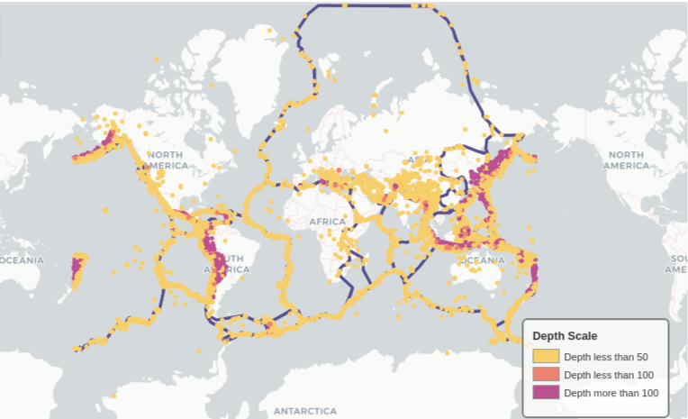
There seem to be some patterns here if you look closely. In places like South America, North America, Southeastern Asia, and in the tectonic boundaries near Oceania, the depth of the earthquake seems to be deeper, the further it is from a boundary. The closer they are the shallower the earthquakes. This might not be easy to grasp intuitively, but that’s the beauty of Data Science, you get unexpected results.

End Notes

Our analysis showed that :

Seismic activities were of relatively high magnitude from 1965 to the early 1970s all around the globe.

Establishments and areas around tectonic plate boundaries are more prone to Earthquakes.

The Depth of Earthquakes decreases in shallowness, as the distance from plate boundaries increases.

The media shown in this article are not owned by Analytics Vidhya and is used at the Author’s discretion.