This article was published as a part of the Data Science Blogathon

The Tech industry is filled with buzz words like “Neural Networks”, “Deep Learning” and “Artificial Intelligence”. But what is it? How is it different from machine learning and why does it resemble the neurons present in our brains?
In this article, we’ll answer these basic questions and build a basic neural network to perform linear regression.
What is a Neural Network?
The basic unit of the brain is known as a neuron, there are approximately 86 billion neurons in our nervous system which are connected to 10^14-10^15 synapses. Each neuron receives a signal from the synapses and gives output after processing the signal. This idea is drawn from the brain to build a neural network.
Each neuron performs a dot product between the inputs and weights, adds biases, applies an activation function, and gives out the outputs. When a large number of neurons are present together to give out a large number of outputs, it forms a neural layer. Finally, multiple layers combine to form a neural network.
Neural Network Architecture
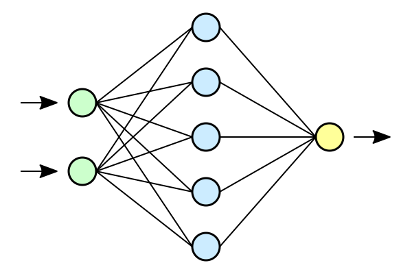
Neural networks are formed when multiple neural layers combine with each other to give out a network, or we can say that there are some layers whose outputs are inputs for other layers.
The most common type of layer to construct a basic neural network is the fully connected layer, in which the adjacent layers are fully connected pairwise and neurons in a single layer are not connected to each other.
In the figure given above, neural networks are used to classify the data points into three categories.
Naming conventions. When the N-layer neural network, we do not count the input layer. Therefore, a single-layer neural network describes a network with no hidden layers (input directly mapped to output). In the case of our code, we’re going to use a single-layer neural network, i.e. We do not have a hidden layer.
Output layer. Unlike all layers in a Neural Network, the output layer neurons most commonly do not have an activation function (or you can think of them as having a linear identity activation function). This is because the last output layer is usually taken to represent the class scores (e.g. in classification), which are arbitrary real-valued numbers, or some kind of real-valued target (e.g. In regression). Since we’re performing regression using a single layer, we do not have any activation function.
Sizing neural networks. The two metrics that people commonly use to measure the size of neural networks are the number of neurons, or more commonly the number of parameters.
Libraries
We’re going to use three basic libraries for this model, numpy, matplotlib, and TensorFlow.
- Numpy- This adds support for large, multi-dimensional arrays and matrices, along with a large collection of high-level mathematical functions. In our case, we’re going to generate data with the help of Numpy.
- Matplotlib- This is a plotting library for Python, we’ll visualize the final results using graphs in Matplotlib.
- Tensorflow- This library has a particular focus on the training and inference of deep neural networks. We can directly import the layers and train, test functions without having to write the whole program.
import numpy as np
import matplotlib.pyplot as plt
import tensorflow as tf
Generating Data
We can generate our own numerical data for this process using the function np.unifrom() which generates uniform data. Here, we’re using two input variables xs and zs, adding some noise to randomly spread the data points, and finally, the target variable is defined as y=2*xs-3*zs+5+noise. The size of the dataset is 1000.
observations=1000
xs=np.random.uniform(-10,10,(observations,1))
zs=np.random.uniform(-10,10,(observations,1))
generated_inputs=np.column_stack((xs,zs))
noise=np.random.uniform(-10,10,(observations,1))
generated_target=2*xs-3*zs+5+noise
After generating the data, save this in a .npz file, so that it can be used for training.
np.savez('TF_intro',input=generated_inputs,targets=generated_target)
training_data=np.load('TF_intro.npz')
Our target is to get the final weights as close to the actual weights, i.e. [2,-3].
Defining the model
Here, we’re going to use TensorFlow dense layer to make the model and import the optimizer stochastic gradient descent from Keras.
A gradient is the slope of a function. It measures the degree to which one variable changes with the changes of another variable. Mathematically, gradient descent is a convex function whose exit is the partial derivation of a set of parameters of its inputs. The greater the gradient, the steeper the slope.
From an initial value, Gradient Descent is run iteratively to find the optimum parameter values to find the minimum possible value for the given cost function. The word “stochastic” refers to a random probability system or process. Thus, in Stochastic Gradient Descent, some samples are randomly selected, rather than the data set for each iteration.
Since, The input has 2 variables, input size=2, and output size=1.
We’ve set the learning rate to 0.02, which is neither too high nor too low, and epoch value=100.
input_size=2
output_size=1
models = tf.keras.Sequential([
                             tf.keras.layers.Dense(output_size)
                            ])
custom_optimizer=tf.keras.optimizers.SGD(learning_rate=0.02)
models.compile(optimizer=custom_optimizer,loss='mean_squared_error')
models.fit(training_data['input'],training_data['targets'],epochs=100,verbose=1)
Getting Weights and Bias
We can print the predicted values of weights and biases and also store them.
models.layers[0].get_weights()
[array([[ 1.3665189],
        [-3.1609795]], dtype=float32), array([4.9344487], dtype=float32)]
Here, the first array represents the weights and the second array represents the biases. We can clearly observe that the predicted values of weights are very close to the actual value of weights.
weights=models.layers[0].get_weights()[0]
bias=models.layers[0].get_weights()[1]
Prediction and Accuracy
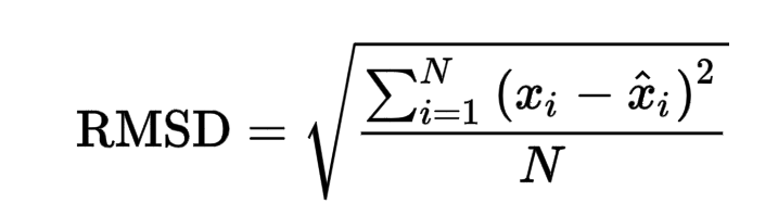
After prediction using the given weights and biases, a final RMSE score of 0.02866 is obtained, which is pretty low.
RMSE is defined as Root mean squared error. Root mean squared error takes the difference for each observed and predicted value. The formula for RMSE error is given as:
https://www.google.com/search?q=rmse+formula&oq=RMSE+form&aqs=chrome.0.0i433j0j69i57j0l7.4779j0j7&sourceid=chrome&ie=UTF-8
 |
|
|
|
 |
|
|
|
 |
|
|
|
 |
|
|
out=training_data['targets'].round(1)
from sklearn.metrics import mean_squared_error
mean_squared_error(generated_target, out, squared=False)
If we plot the predicted data on a scatter plot, we get a graph like this:
plt.scatter(np.squeeze(models.predict_on_batch(training_data['input'])),np.squeeze(training_data['targets']),c='#88c999')
plt.xlabel('Input')
plt.ylabel('Predicted Output')
plt.show()
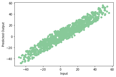
Yay! Our model trains properly with very little error. This is the end of your very first neural network. Note that every time we train the model we may get the different value of accuracy, but they’ll not differ much.
Thank you for reading! You can contact me at [email protected].


