This article was published as a part of the Data Science Blogathon.
Introduction
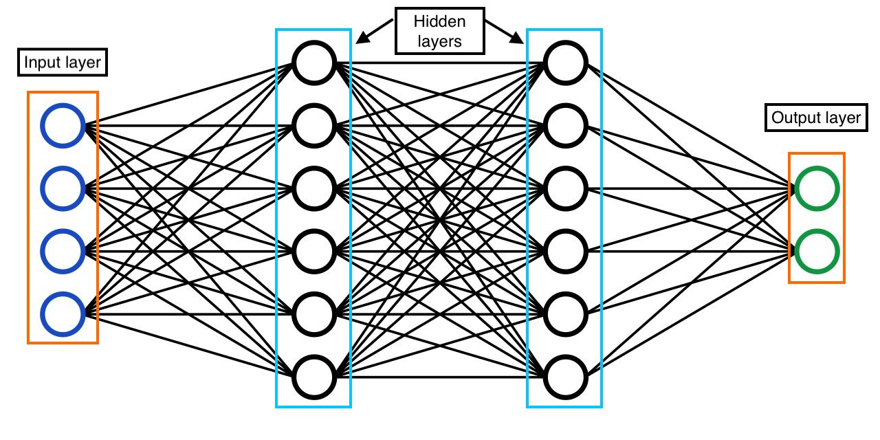
Deep learning is a branch of Machine learning where higher levels of features from the data can be extracted using an Artificial neural network inspired by the working of a neural system in the human body. A neural network is a combination of multiple layers where each layer consists of multiple units, and these layers are mainly categorized into three sections 1. An input layer, 2. Hidden layer(s), and 3. Output layer. A neural network is said to be dense layered NN. When each unit from one layer is connected to every other unit in the next layer then, it is said to be a dense, layered neural network.
The Idea of Neural Network – Perceptron
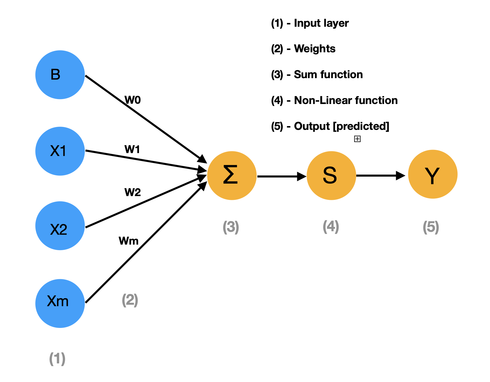
The above diagram represents the perceptron model where we have an input layer, weights respective to each unit, and SUM function [X1*W1+X2*W2+…..+XmWm] where X1 X2…Xm represents input features and W1 W2…Wm represents weights, A non-linear function which we will discuss more, and finally, the predicted output. Mathematically we write the same diagram as below:
ŷ = g (W0 + ∑ Xi * Wi)
= g (Wo + XT. W), Where XT= [X1,…….,Xm] & W = [W1,…….,Wm]T
In a perceptron, each input is multiplied by its respective weight and taken as a sum, then passed to a non-linear function, giving us a result between zero and one. Three non-linear functions are generally used 1. Sigmoid function, 2. Hyperbolic tangent, 3. Rectified Linear unit (ReLu). ReLU is a commonly used non-linear function in practice. Linear functions aren’t used because linear functions produce linear decisions on data no matter how much the data size is. At the same time, the non-linear function allows for the approximation of complex functions and gives better predictions.
Perceptron – Dense Neural Network
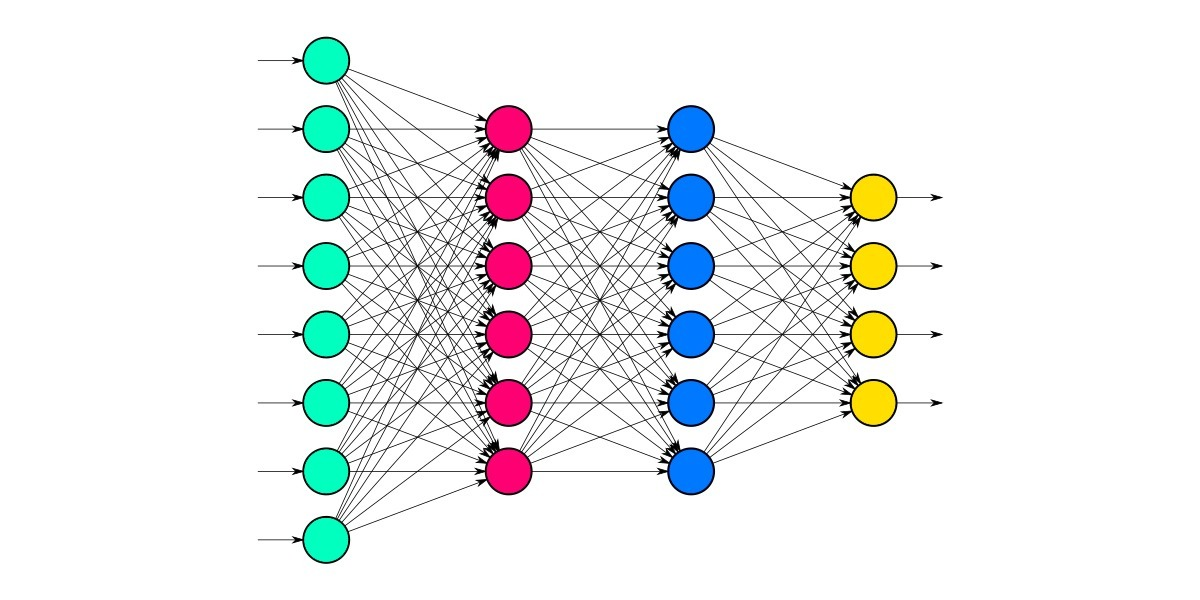
source: https://medium.com/appengine-ai/
When multiple perceptrons connect with multiple combinations, it is called a fully connected neural network. The above picture represents a fully connected neural network, i.e., (each unit in one layer is connected with every other unit in the other layer). In a Neural network, there are certain parameters, when altered, that give better results, and they are called Hyperparameters. Loss function and Optimizer are the main hyperparameters in a neural network. Let’s see each of them with a detailed explanation. Say we have a neural network with one unit in the output layer; after passing the features of the data in the input layer, we get a predicted output accordingly. When we compare our model’s predicted result with our actual label data, there will be a difference which is termed a loss. A model is said to be efficient when the loss is minimized to the lowest possible value. To measure the loss of a model, we mainly use two metrics 1. MAE 2. MSE
Calculating Loss
Mean absolute error (MAE) is one of the loss functions calculated by the ratio of the sum of the absolute difference between actual output and predicted output to the total number of input values. This is generally used while working on a regression model and to make outliers neglected. Mean squared error (MSE) is calculated by the sum of the squared difference of predicted output and actual output to the total number of input values. This is used when large errors are more significant than smaller errors. There is another loss function that is used called Huber, which is the combination of both MAE and MSE. This is widely used for robust regression problems and this is less sensitive to outliers than MSE.
MAE:
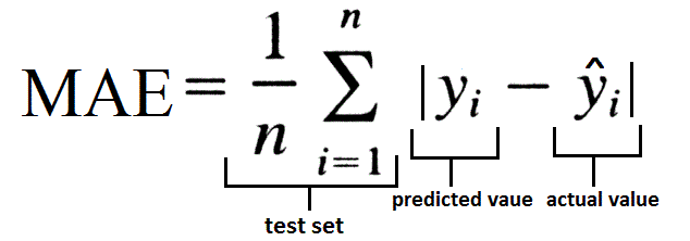
source: https://www.datavedas.com/model-evaluation-regression-models/
MSE:
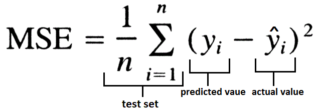
source: https://www.datavedas.com/model-evaluation-regression-models/
So, if the loss is minimized to the least, then the model is perfect enough to say that the neural network made is ready to use. Loss is a function of the network of weights i.e, L( f(X(i); W), Y(i)). To understand the loss function, let’s brush up on our higher math concept called GRADIENTS.
Loss Optimization
The gradient is a vector of partial derivatives used for multivariable functions, whereas the concept of slope (a scalar quantity) is used for single variable functions. NOTE: Gradient & slope looks the same, but they are not !!. The gradient of a function gives a vector and tells the direction to reach the maximum global value of the function. In general, terminology, if you stand at a point (X0, Y0, Z0,….) in the input space f, the vector Del F(X0, Y0, Z0,…) tells you in which direction you should travel to maximize the value of function most rapidly.
Let’s come back to our process of loss optimization. When we apply the gradient, as said above to the loss function, it will take us to the value where our loss is more maximized. So to avoid that, we will go opposite our gradient’s direction and find the local minima value of the loss function. This process happens for a set of iterations to find the best possible weights for our model. Once we reach our local minima we will take the corresponding weights that give the lowest value. In Machine learning or Deep learning, we set our ‘epochs’ to a finite value, which means we train the model by updating the weights in each iteration to minimize the loss. Now we will look into an example given below.
source: https://www.gmcindia.in/
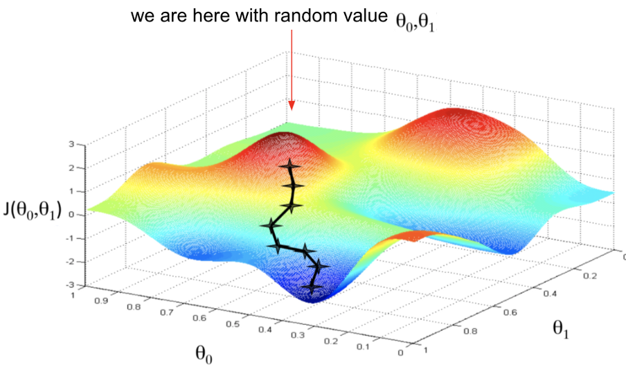
For instance, we have a multi-variable loss function J(W0, W1) of weights W0 and W1 as inputs. Now let’s frame an algorithm for loss optimization taking the above graph as a reference.
Algorithm
Step 1: Take any two points W0, W1 randomly
Step 2: Loop until finds the lowest possible loss:
Step 3: Compute gradient for the function J(W0, W1), This gradient tells the direction to maximize the loss. So we will go exactly opposite the direction to get minimum loss.
Step 4: Updating weights (includes the process of learning rate and backpropagation )
Step 5: Return weights
This is how we update our weights for every iteration to make our model’s loss minimal, and this process is called Gradient Descent. A viral algorithm called ‘Stochastic Gradient Descent’ SGD is frequently used in practice mainly for regression models, which is very similar to the process that is discussed above but in SGD, while computing the gradient of the loss function, we pick a subset, say B (which is a subset of the whole dataset) as batches to compute gradient and update accordingly. Mini batches lead to faster training and can parallelize computation plus achieve significant speed increase on GPUs. Adam is also another loss optimizer that is used in practice.
Model Fitting
The final step to check the neural network on how well it got trained is by the method called ‘Fitting.’ The model fitting has three possible cases (under-fit, ideal-fit, and over-fit). When the model can’t fully learn the data, it is called underfitting in other words, underfitting occurs when a model is unable to effectively identify the relation between input and output values. When the model learns the data perfectly, it is called an ideal fit. When the model is trained with too many complex parameters and doesn’t generalize well then it is called overfitting in other words, when a model is overfitted, the data is too closely matched.
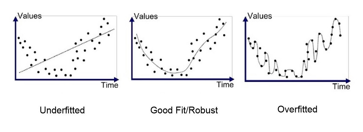
source: https://medium.com/@minions.k/
To adjust this problem, a technique called Regularization is proposed which constrains the optimization problem to discourage complex models. This helps to improve the generalization of a model on unseen data. There are two techniques that can be implemented- Dropout and Early stopping.
In the Dropout technique during training, the units in the layer are randomly set activation to zero. It means disabling the units to make the model look into different patterns. In the Early stopping technique, the training gets stopped before a chance to overfit the model. Look at the below image for a better understanding. In the below graph training is stopped at a point where the value of testing error raises.
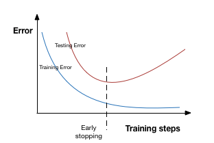
source: https://www.analyticsvidhya.com/blog/
Coding for Neural Network
Let’s get started !!
Importing necessary libraries
import tensorflow as tf
Three important steps in modelling a neural network:
- Creating a model – Define input & output layers and hidden layers of the deep learning model.
- Compiling the model – Define the loss function, i.e., (how wrong the model is), the optimizer( which tells how to improve the patterns in learning), and evaluation metrics (to interpret the performance of our model).
- Fitting the model – Let the model try to find patterns between x and y (features and labels), respectively.
Let’s write the code which matches the architecture of the neural network in Fig-8
#set random seed
tf.random.set.seed(42)
#1. Create the model
model = tf.keras.Sequential([
tf.keras.layers.Dense(6, input_shape = (4, ), activation = 'relu'),#Hidden layer
tf.keras.layers.Dense(6, activation = 'relu'),# Hidden layer
tf.keras.layers.Dense(2, activation = 'relu')])# Output layer#2. Compile the model
model.compile(loss = tf.keras.losses.mae,
optimizer = tf.keras.optimizers.SGD(),
metrics = ["mae"])#3. Fit the model
model.fit(x_train, y_train, epochs=100, verbose=0)Let’s understand the code line by line and see if we achieved the neural network as in Fig – 8. In the first line, we randomly set the seed with a constant value so that it initializes whenever the model runs with the same weights. The above code is a basic block of code that creates a neural network model.
Explanation
1. In the first step, we use the Sequential function to form the layers in a stacked /sequential manner. In the first layer, 6 represents the number of units in the layer. input_shape = (4, ) creates an input layer with 4 units, and activation is assigned as relu.
2. Our model is compiled with three parameters in the second step. Loss tells the model to use certain metrics to calculate the loss. In our code, we used the MAE method. The optimizer tells the model to reduce the loss value and use the best possible updated weights in the given number of epochs. List of metrics that the model will consider while being trained and tested.
3. In the last step, the model is trained using model.fit, where testing and training sets are passed as parameters. To train the model, epochs=100 will iterate for hundred times to reduce the loss value by adjusting the weights.
Conclusion
In this article, we have seen the architecture of neural networks, their loss functions, an algorithm for the optimizer, model fitting, and training. Taking this as a base, we can understand other neural network algorithms like RNN, which is used for sequential input like sentences, and CNN, which is used for image data. The field of Deep learning is vast and growing day by day.
Takeaways:
- Perceptron is the first idea to develop a neural network and is inspired by the human neural system
- The output of a unit results by applying a non-linear function to the value, which is a multiplication of weights and input values.
- Loss can be rectified by using loss optimizers like SGD, which uses a methodology of backpropagation. Certain metrics like MAE & MSE can measure loss.
- Finally, the model is fitted to the data for model training.
- The media shown in this article is not owned by Analytics Vidhya and is used at the Author’s discretion.
If you’re eager to dive deeper and explore the intricacies of these powerful algorithms, check out our detailed guide on the working of neural networks. Expand your knowledge and stay ahead in the evolving world of Deep Learning!
I'm Naru Venkata Pavan Saish, a hardworking and dedicated student pursuing Btech 3rd year in CSE with a data science specialization in VIT Vellore. Interested in Data science and Machine learning fields. Enthusiastic writer and a keen interest in developing code.


