A Guide To Monte Carlo Simulation!

This article was published as a part of the Data Science Blogathon

Introduction

Monte Carlo simulation is a computational algorithm that makes use of repeated random sampling to get the likelihood of a range of an unknown quantity. Sounds difficult! don’t worry, we will explore this in-depth in this article

A Brief History:

The Monte Carlo Method was invented by John Neumann and Ulam Stanislaw to improve decision-making under uncertain conditions. It was named after a well-known casino town Monte Carlo called Monaco since the element of chance is core to the modelling approach as it is similar to a game of roulette.

In easy words, Monte Carlo Simulation is a method of estimating the value of an unknown quantity with the help of inferential statistics. You need not dive deep into inferential statistics to have a strong grasp of Monte Carlo simulation’s working. However, this article will go only through those points of inferential statistics which will be relevant to us in the Monte Carlo Simulation.

Inferential Statistics deals with the population which is our set of examples and sample, which is a proper subset of the population. The key point to notice is that a random sample tends to exhibit the same characteristics/property as the population from which it is drawn.

We will go through an example to understand the working of the Monte Carlo simulation.

We aim to estimate that how likely is it to get ahead if we flip a coin an infinite number of times.

1. Let’s say we flip it once and get ahead. Will we be confident to say that our answer is 1?

2. Now we flipped the coin again and it again appeared head. Are we sure that the next flip will also be ahead?

3. We flipped it over and over again, let’s say 100 times, and strangely head appears every time. Now, do we need to accept the fact that the next flip will result in another head?

4. Let us just change the scenario and assume that out of 100 flips 52 resulted in the head will rest 48 came to be tails. Is the probability of the next flip resulting in the head is 52/100? Given the observation, it’s our best estimate, But the confidence will be still low.

Why is there a difference in Confidence Level?

It is important to know that our estimate depends upon two things

1. Size: the size of the sample (e.g., 100 vs 2 in cases 2 and 4 respectively)

2. Variance: variance of the sample (all the results as head versus 52 heads as in case 3 and 4 respectively)

3. As the Variance of the observation grows (case 3 and 4), there comes a need for larger observation (as in cases 2 and 4) to have the same degree of confidence.

We will be now simulating a Roulette game (python):
Roulette is a game in which a disk with blocks (half red and half black) in which a ball can be contained, is spin with a ball. We need to guess a number and if the ball land up in this number, then it’s a win, and we win an amount of (paid amount for one slot
) X (no. of total slots in the machine).

100 spins of Roulette
Expected return betting 5 = -100.0%
100 spins of Roulette
Expected return betting 5 = 42.0%
100 spins of Roulette
Expected return betting 5 = -26.0%
1000000 spins of Roulette
Expected return betting 5 = -0.0546%
1000000 spins of Roulette
Expected return betting 5 = 0.502%
1000000 spins of Roulette
Expected return betting 5 = 0.7764%

Law of Large Numbers

 

In repeated independent tests with the constant probability p of the population of a particular outcome in each test, the probability that the outcome occurs i.e. obtained from the samples differs from p converges to zero as the number of trials goes to infinity.

It simply means that if deviations (Variance) occur from the expected behaviour (probability p), in the future these deviations are likely to be evened out by the opposite deviation.

Now let’s talk about an interesting incident that took place on 18 August 1913, at a casino in Monte Carlo. In roulette, black came up a record twenty-six times in succession, and there arose a panic to bet red (so to even out the deviation from expected behaviour)

Let’s analyze this situation mathematically

1. Probability of 26 consecutive reds = 1/67,108,865

2. Probability of 26 consecutive reds when previous 25 rolls were red =1/2

Regression to Mean

1. Following an extreme random event, the next random event is likely to be less extreme so that the mean is maintained.

2. E.g. if the roulette wheel is spun 10 times and reds come every time, then it is an extreme event =1/1024 and it is likely that in the next 10 spins we will get less than 10 reds, But the average number is 5 only.

So, as we look at the mean of 20 spins, it will be closer to the expected mean of 50% reds than to the 100% as of in the first 10 spins.

Now time to face some reality.

Sampling space of possible Outcomes

1. It is not possible to guarantee perfect accuracy through sampling and also cannot say that an estimate is not precisely correct

We face a question here that how many samples are required to look at before we can have significant confidence in our answer?

It depends upon the variability in underlying distribution.

Confidence levels and Confidence Intervals 

As in a real-life situation, we cannot be sure of any unknown parameter obtained from a sample for the whole population so we make use of confidence levels and confidence intervals.

The confidence interval provides a range that the unknown value is likely to be contained with the confidence that the unknown value lays strictly within that range.

For example, the return for betting on a slot 1000 times in roulette is -3% with a margin error of +/- 4% with a 95% level of confidence.

It can be further decoded as we conduct an infinite trial of 1000,

The expected average/mean return would be -3%

The return would roughly vary between +1% and -7% that also 95% of the time.

Probability Density Function (PDF).

 

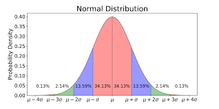
Distribution is usually defined by the probability density function (PDF). It is defined as the probability that the random variable lying between an interval.

The area under the curve between the two points of PDF is the probability of the random variable falling within that range.

Let’s conclude our learning by an example:

Let’s say there is a deck of shuffled cards and we need to find the probability of getting 2 consecutive kings if they lay down the cards in the order they are placed.

Analytical method:

P (at least 2 consecutive kings) = 1-P (no consecutive kings)

=1-(49! X 48!)/((49-4)! X52!) = 0.217376

By Monte Carlo Simulation:

 

Steps

1. Repeatedly select the random data points: Here we assume the shuffling of the cards is random

2. Performing deterministic computation. A number of such shuffling and finding the results.

3. Combine the results: Exploring the result and ending with our conclusion.

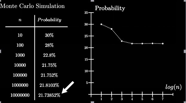
By Monte Carlo method we achieve near exact solution as of analytical method.

Advantages of Monte Carlo Simulation

• Easy to implement and it gives statistical sampling for numerical experiments using the computer.
• Provides us with satisfactory approximate solutions to computationally expensive mathematical problems.
• It can be used for deterministic as well as stochastic problems.

Disadvantages of Monte Carlo Simulation

• It is sometimes time-consuming as we have to generate a large number of samplings to get the desired satisfactory output.
• The results obtained from this method are only the approximation of the true solution and not the exact solution.

About the Author

I am Dinesh Junjariya a Btech student from IIT Jodhpur.

For any suggestions please comment down below.