This article was published as a part of the Data Science Blogathon.
Introduction
This article aims to introduce Monte Carlo Simulation for variable uncertainty analysis. Monte Carlo can replace the propagation of error because it overcomes the disadvantages of the propagation of error. We will discuss:
- How to perform propagation of error;
- Why use Monte Carlo instead of the propagation of error; and
- The steps of performing Monte Carlo uncertainty.
Let’s start this discussion with simple things. How much does an employee in city A spend on living expenses in one month? There are thousands of employees in city A with different living expenses. To answer the question above, we need to ask a number of employees and record their answers. Those employees will answer differently. Their living expenses will vary in a probability distribution. Even though we do not have the resource to ask all the employees, we can sample a group of, for instance, 50 employees for the survey to represent the population.
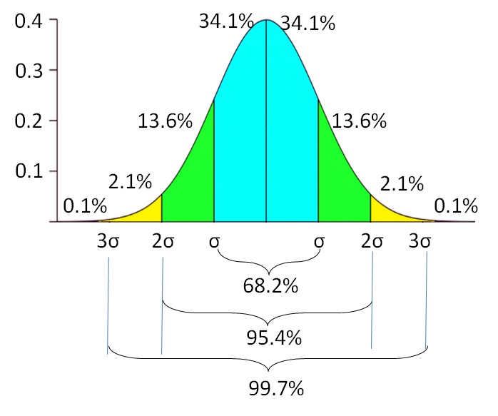
However, we still need a number to represent the overall living expense. Let say we get the average monthly living expense is $2000. Or, another way is to use the median to represent the overall expense. To express other possible living expenses, we can use the standard deviation. For example, the monthly living expense in city A is $2000 ± 500 (average ± standard deviation).
It means that if the data are normally distributed, 68.2% of the employees spend $1500 to $2500. There is another 31.8% of employees spend less than $1500 and more than $2500 for monthly living costs. The probability of the living expense lowers as it is further away from the average. There is a 0.1% probability of finding employees with living expenses less than $500 or more than $3500. The standard deviation reflects the variable uncertainty of the living expense. It indicates the lower and upper extent of the variable, instead of relying on only 1 single value.
Propagation of Error
Given that city A employees have income: $3200 ± 2000, living expense: $2000 ± 500, credit: $180 ± 130, unexpected income or expense: $20 ± 300, and bank interest rate: 0.85 ± 0.35% per month. We want to calculate how much an employee can save in a month. The equation is expressed below:
Saving = (Income – Living_Expense – Credit + Unexpected_Income/Expense) × (1 + Interest)
Monthly saving is calculated as total income deducted by living expenses and credit and added with unexpected income or expenses. After one month, the saving nominal increases due to the bank interest. We will calculate the monthly saving average and the uncertainty. Please observe the following equation on how to calculate the uncertainty.
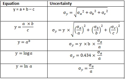
Fig. 2 Propagation of Error
Saving1 = ((3200 ± 2000) - (2000 ± 500) - (180 ± 130) + (20 ± 300)) × (1 + (0.0085 ± 0.0035))

Saving1 = 1040 ± σSaving_1
σSaving_1 = ((20002 + 5002 + 1302 + 20002))0.5

σSaving_1 = 2087
Saving1 ± σSaving_1 = 1040 ± 2087
This calculates the monthly saving after accounting for the bank interest.
Saving = Saving1 × (1 + (0.0085 ± 0.0035))

Saving = (1040 ± 2087) × (1.0085 ± 0.0035)

Saving = 1049 ± σSaving_2
σSaving = 1049 × ((2087/1040)2 + (0.0035/1.0085)2)0.5

σSaving = 1049 × 2.01

σSaving = 2105
Saving ± σSaving = 1049 ± 2105
From the result, we can see that on average people can save $1049 in a month with the uncertainty of $2105. The lower bound of the monthly saving is -$1056 ($1049 – $2105), which is a negative value. The uncertainty itself is 2105 which is 2 times larger than the mean value. If we visualize the graph, we can see that employees’ savings range from -$6000 to $8000. It seems weird because the lower and upper bound are almost balanced. I think, in reality, the saving amount should have higher variability than the deficit amount.
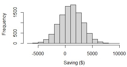
Fig. 3 Visualizing saving in a normal distribution
How is this happening? The problem is with the income data. The income of $3200 ± 2000 has high uncertainty due to the income variability. The uncertainty is more than one-third of the mean value. If we assume this is normal distribution, we will see 4.8% of the population has income under 0, which seems not likely to happen. In fact, income should be always above %0. This problem happens when we assume that all of the variables are normally distributed, but in reality, they are not.
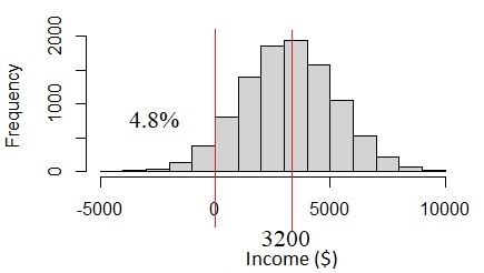
Fig. 4 Normal distribution if income standard deviation is too big
Monte Carlo Simulation
What is the solution? Another way to assess uncertainty is by applying Monte Carlo Simulation. Monte Carlo is originally the name of an administrative area in Monaco. But, the Monte Carlo of our discussion today is statistics material. Monte Carlo can overcome the disadvantage of error propagation. Monte Carlo Simulation, unlike propagation of error, can work on data distribution other than normal distribution and data with big standard deviation.

Fig. 5 Monte Carlo in Monaco. Source: Google Map
Monte Carlo simulation simulates or generates a set of random numbers according to the data distribution and parameters for each variable. After generated, all variables values are calculated using the equation. This sounds a bit more complicated than using propagation of error. But using Data Science tools, such as Python or R, it will be very simple. In this discussion, we will demonstrate using R statistical language.
Steps of Performing Monte Carlo Simulation
1. Check the probability density function of the data distribution
Let say, we examine the data record provided from the survey of 50 respondents. There are many types of probability density functions and we have to determine which one fits our data. The variables with normal distribution are only living expenses and unexpected income or expenses. The income data distribution is positive skew.
In this case, we will treat it as a gamma distribution. This is the reason why the average and propagation of error are not suitable for this data. The other two variables also do not have a normal distribution. The bank interest rate is distributed uniformly ranging from 0.3 to 1.5.
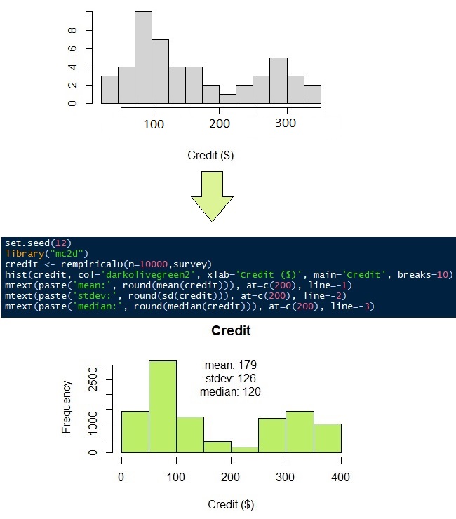
The data distribution of credit loans to pay is quite unique. The data are distributed mostly into two population groups. The first group has lower credit than the second group does. Let say, the data distribution of credit does not fit any probability density function. Then, we will use non-parametric distribution.
2. Generate Monte Carlo Simulation
To generate Monte Carlo Simulation means to generate a set of random numbers with the same data distribution as the original data. To do this, we just set the number of simulations and the distribution parameters according to the distribution type. We set the number of simulations to be 10,000. It means that we will simulate 50 respondents’ data into 10,000 data.
The parameters of the normal distribution are mean/average and standard deviation. We have known the averages ± standard deviations of living expenses and unexpected income or outcome are 2000 ± 500 and 20 ± 300 respectively. Now, we can generate the distributions. In this article, I will use the R language. Of course, other Data Science languages, like Python, also can do it. See that the simulated data has similar, not the same, mean and standard as the input parameters.
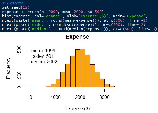
Fig. 6 Normal distribution of living expense
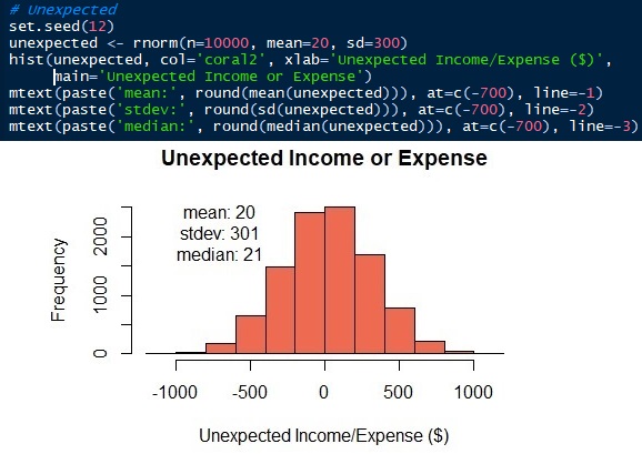
Fig. 7 Normal distribution of unexpected income or expense
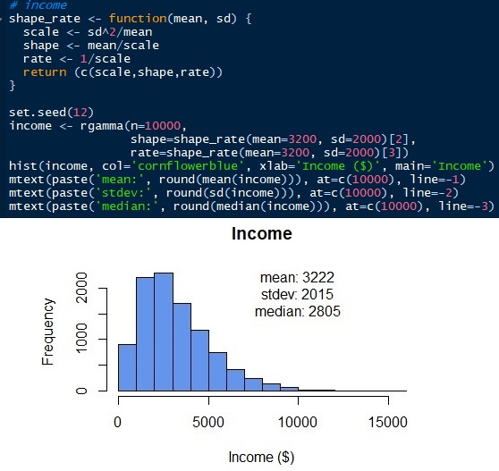
To generate gamma distribution, we need to know other parameters. Unlike the normal distribution, gamma distribution has scale, shape, and rate as the parameters. But we can get those parameters with mean and standard deviation (sd). Scale = sd2/mean. Shape = mean/scale. Rate = 1/scale. Then, we can simulate the gamma distribution for employees’ income as below. Gamma distribution can only have positive values. There is no value under 0 as all employees’ income should be a positive number. Normal distribution would give negative values if the standard error is too big. See that the simulated distribution has a mean and standard deviation of 3222 and 2015 respectively, which are close to the original input parameters. But, we have a median of 2805. The median of the gamma distribution, unlike the normal distribution, is far from the mean.
Monthly credit to pay, as mentioned above, does not have a suitable probability density function. Have a look at the responses of 50 surveys in Figure 9 (grey histogram). It looks like most people have to pay their credit of $100 and $300. To simulate the 50 observations into 10,000 observations, we can use non-parametric distribution. As its name suggests, non-parametric distribution does not require parameters, such as mean, standard deviation, shape, or rate like normal and gamma distributions do. It requires only the original data.
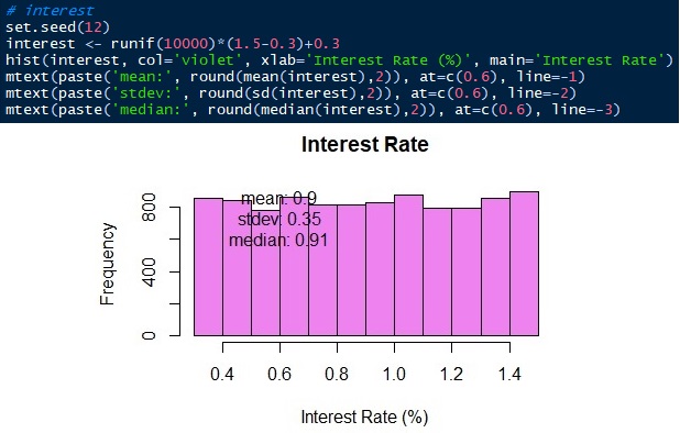
The last variable to simulate is the bank interest rate. The bank interest rate ranges from 0.3 to 1.5 uniformly. We will simulate 10,000 observations ranging from 0.3 to 1.5 with the same probability.
3. Combining the Monte Carlo Simulations
The last step is to combine the Monte Carlo Simulations by using the equation to calculate the monthly saving. To do this, we just need to put all of the simulations together in a table. Then, we can calculate 10,000 rows of monthly savings. The result is $1073 ± 2052, not far different from the propagation of error. But, Monte Carlo Simulation shows the probability density. We can see that the saving median is $666 and the data range from $2000 to 10000.
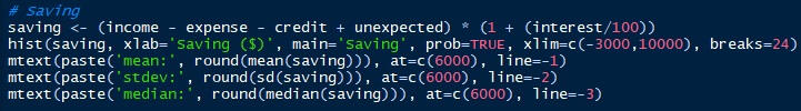
Table 1 – Combining Monte Carlo Simulations
Now, let’s look at another example with spatial and temporal variability. The task is to calculate the surface runoff of a watershed. Watershed is the boundary of surface water hydrology. All of the rainfall which falls under the watershed will not cross outside the boundary. Some of the rainfall infiltrates the soil according to the soil particle size and land cover type. The water that does not infiltrate into the soil is called surface runoff. The surface runoff will stream to the river as the river discharge.
The following table shows the monthly rainfall intensity in a year and the runoff coefficient in a 1.5 km2 watershed. Uncertainty can happen from spatial and temporal heterogeneity. Rainfall and runoff coefficient (due to soil and land cover type) varies spatially in the watershed. The watershed rainfall is measured by a number of rain gauges. They give average rainfall with uncertainty due to spatial distribution. The land cover distribution also gives the uncertainty of the runoff coefficient.
A runoff coefficient is the ratio of rainfall that does not infiltrate the soil and becomes surface runoff. Forest or coarse soil type has a low runoff coefficient. Settlements or houses have a high runoff coefficient. Converting land cover from the forest into settlements increases the runoff coefficient because more ratio of rainwater will be a surface runoff.
Temporal variability also happens as rainfall in wet and dry seasons is different. Land cover change over time also causes the runoff coefficient temporal variability. Other sources of uncertainty are the quality of measurement tools, measurement methods, environmental conditions, and other unexplained conditions due to a lack of knowledge.
| Month | Rainfall (mm/month) | Runoff Coefficient | Area (km2) |
| Jan | 320 ± 37 | 0.3 ± 0.2 | 1.5 |
| Feb | 350 ± 59 | 0.3 ± 0.2 | 1.5 |
| Mar | 205 ± 26 | 0.4 ± 0.1 | 1.5 |
| Apr | 170 ± 41 | 0.4 ± 0.1 | 1.5 |
| May | 106 ± 48 | 0.4 ± 0.1 | 1.5 |
| Jun | 91 ± 32 | 0.4 ± 0.1 | 1.5 |
| Jul | 77 ± 16 | 0.4 ± 0.1 | 1.5 |
| Aug | 52 ± 15 | 0.7 ± 0.2 | 1.5 |
| Sep | 100 ± 50 | 0.7 ± 0.2 | 1.5 |
| Oct | 120 ± 46 | 0.7 ± 0.2 | 1.5 |
| Nov | 253 ± 45 | 0.7 ± 0.2 | 1.5 |
| Dec | 210 ± 48 | 0.7 ± 0.2 | 1.5 |
The equation is surface runoff = rainfall intensity × runoff coefficient × watershed area. All distribution is simulated using a gamma distribution. The average monthly surface runoff is 124,000 ± 30 m3/month. The median is 120,000 m3/month.
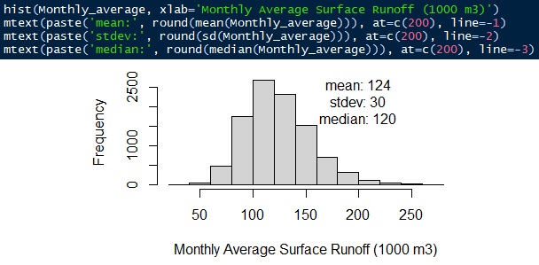
Fig. 12 Monthly average surface runoff
About Author
Connect with me here https://www.linkedin.com/in/rendy-kurnia/
The media shown in this article are not owned by Analytics Vidhya and is used at the Author’s discretion.
A Data Science professional with seasoned specializations in Machine Learning development and Geo-spatial analysis. Hold the TensorFlow Developer Certificate. Have strong work experience in: - delivering meaningful data-driven insights to support business goals, - automating data processing, - data analysis (tabular, time series, text/NLP, and image), - descriptive and inferential statistical analysis, - GIS or spatial data analysis, - data visualization and dashboard development, - Machine Learning modeling (regression, classification, clustering, dimensionality reduction, time series forecasting, recommender engine) - Deep Learning or Artificial Intelligence (regression and classification with MLP, image classification with CNN, time series forecasting with LSTM, text classification with LSTM) - Hugging face: transformers, fine-tuning - Large Language Models (LLM) - Stable Diffusion - web application development, - developing APIs, etc.


