This article was published as a part of the Data Science Blogathon
In the last blog, we discussed what an Artificial Neural network is and how does it work. If you have not gone through it, please refer to the attached article. Today, we are going to see the practical implementation of ANN on the Unstructured data.
Unstructured data can be text, images, videos, audios, basically the data which is not in a defined or structured format. There are no predefined rows, columns, values, or features in the Unstructured data, and is messier than structured data. Deep learning models are designed in such a way that they mimic the human brain capacity and are therefore more robust in solving these types of problems.
Here, We are going to use MNIST Handwritten Digit data which contains the images of handwritten digits. It will be a step by step implementation with an explanation so keep on reading 🙂
The first step in building any model is importing the libraries and reading data.
#importing libraries
import numpy as np
import pandas as pd
import matplotlib.pyplot as plt
import seaborn as sns
# Ignore the warnings
import warnings
warnings.filterwarnings("ignore")
Reading the data
#loading MNIST dataset
from tensorflow.keras.datasets import mnist
(X_train,y_train) , (X_test,y_test)=mnist.load_data()
X_train and X_test contain greyscale RGB codes (from 0 to 255) while y_train and y_test contain labels from 0 to 9 which represents which number they actually are.
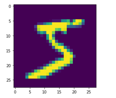
#visualizing the image in train data
plt.imshow(X_train[0])
#visualizing the first 20 images in the dataset


for i in range(20):

    #subplot

    plt.subplot(5, 5, i+1)

    # plotting pixel data

    plt.imshow(X_train[i], cmap=plt.get_cmap('gray'))

# show the figure

plt.show()
Checking the shape of train and test data
print(X_train.shape)
print(X_test.shape)
Output:
(60000, 28, 28)
(10000, 28, 28)
Train data (X_train) has 60000 images of size 28*28 and Test data (X_test) has 10000 images. Each image is 2D and its pixel ranges from 0 to 255. You can check by printing the below code.
# the image is in pixels which ranges from 0 to 255
X_train[0]
As a part of pre-processing step, we need to convert these images from 2D to 1D to feed them into the Artificial Neural network model, for which we are going to use the reshape function. After flattening the images the shape of the image will change to:
X_train_flat=X_train.reshape(len(X_train),28*28)

X_test_flat=X_test.reshape(len(X_test),28*28)

#checking the shape after flattening

print(X_train_flat.shape)

print(X_test_flat.shape)
Output:
(60000, 784)
(10000, 784)
Check the new representation of the image using the below code:
#checking the representation of image after flattening
X_train_flat[0]
The next step in pre-processing is Normalizing the pixel values which will be fed into the model. As we Standardize or normalize our data for Machine learning model building, the same way we normalize the data for Deep learning model building. Here our data is in pixel format, so we will normalize it in such a way that it ranges from 0-1.
#normalizing the pixel values
X_train_flat=X_train_flat/255
X_test_flat=X_test_flat/255
#print this code to check the pixel values after normalization
X_train_flat[0]
After all the preprocessing, now it’s time to build the model.
A Deep Learning model is built in the following steps:
We will be building a very simple model first in which there will only be an input layer, an output layer, and an activation function applied to it.
#Building a simple ANN model without hidden layer
#importing necessary libraries
from tensorflow.keras.models import Sequential
from tensorflow.keras.layers import Dense
#Step 1 : Defining the model
model=Sequential()
model.add(Dense(10,input_shape=(784,),activation='softmax'))
In the above code, we are defining the model using the Sequential() function and adding the input shape and output layer to it. With that, we are using the softmax activation function as we have a multi-class classification problem and have more than two class labels.
#Step 2: Compiling the model
model.compile(loss='sparse_categorical_crossentropy',optimizer='adam',metrics=['accuracy'])
In Step 2, we are compiling the model using the loss, optimizer, and metrics. Loss, we are using sparse_categorical_crossentropy as there are more than two labels in our dataset. For the optimizer, we have used Adam for updating the weights, to achieve minimum losses in the model and Accuracy as a metric.
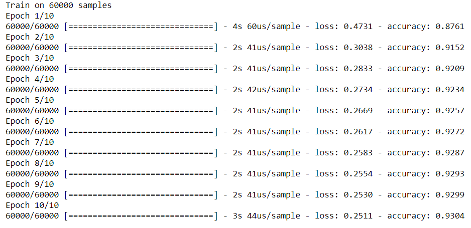
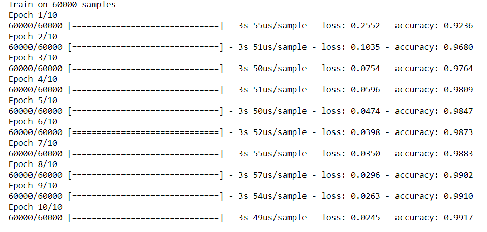
#Step 3: Fitting the model
model.fit(X_train_flat,y_train,epochs=10)
Here we are fitting the defined model on train and test datasets with the specified number of iterations. One complete process of forwarding and backpropagation of the training dataset is considered as one epoch.
Output:
From the above output, we can see that the training accuracy is 93% and the loss is 0.25. Let’s evaluate the model on test data as well.
#Step 4: Evaluating the model
model.evaluate(X_test_flat,y_test)

For the test accuracy, we got 92% and the loss is 0.28
#Step 5 :Making predictions
y_predict = model.predict(X_test_flat)
y_predict[3] #printing the 3rd index
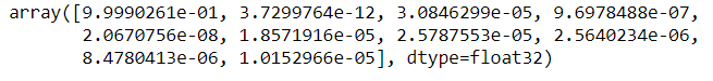
In the above output, we are getting 10 values as our target variable has 10 labels (0 to 9). The value with the highest probability is the predicted output. To get the value with the highest probability we will be using the below code.
# Here we get the index of the maximum value in the above-encoded vector.
np.argmax(y_predict[3])
The output of the above code is 0 which means the predicted digit is 0.
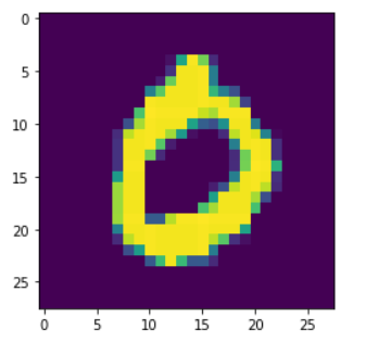
Now we have to check whether our predicted output is the same as our actual output. For the same, we are checking the third index image in the test data and as we have got 0 in the output, this implies that our prediction is the same as the actual.
#checking if the predicting is correct
plt.imshow(X_test[3])
y_predict_labels=np.argmax(y_predict,axis=1)
#Confusion matrix
from sklearn.metrics import confusion_matrix
matrix=confusion_matrix(y_test,y_predict_labels)
#visualizaing confusion matrix with heatmap
plt.figure(figsize=(10,7))
sns.heatmap(matrix,annot=True,fmt='d')
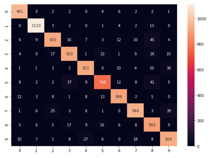
model2=Sequential()
#adding first layer with 100 neurons
model2.add(Dense(100,input_shape=(784,),activation='relu'))
#second layer with 64 neurons
model2.add(Dense(64,activation='relu'))
#third layer with 32 neurons
model2.add(Dense(32,activation='relu'))
#output layer
model2.add(Dense(10,activation='softmax'))
#compliling the model
model2.compile(loss='sparse_categorical_crossentropy',optimizer='adam',metrics=['accuracy'])
#fitting the model
model2.fit(X_train_flat,y_train,epochs=10)
#evaluating the model
model2.evaluate(X_test_flat,y_test)

In this model i.e model 2, training accuracy is 99% and test accuracy is 97%. The loss of train and test is 0.02 and 0.1 respectively. You can print the confusion matrix of model 2 to check the Actual VS Predicted labels.
We are done with the basic neural network model building. In this article, I have guided you step by step to build a Neural network model. In the upcoming blog, we will talk about various other details and steps which is required while building a model such as Dropout and Hyperparameter tuning. So stay tuned for my next blog 🙂
I am Deepanshi Dhingra currently working as a Data Science Researcher, and possess knowledge of Analytics, Exploratory Data Analysis, Machine Learning, and Deep Learning. Feel free to content with me on LinkedIn for any feedback and suggestions.
Lorem ipsum dolor sit amet, consectetur adipiscing elit,


Thank you for sharing this use case and demonstrating how lean it can be done! A question: Why do call this use case "on Unstructured Data" ? Due to my intuition I would call images as "structured data". Thank you, Peter