Introduction-
With the rise of social media in recent years, there has been a surge in interest in automatically identifying users based on their informal content. In this context, the research of other aspects intrinsic to users, such as political inclinations, personality, and gender, as well as the categorization of users in demographic categories such as age, ethnicity, origin, and race has gained a lot of interest notably based on Twitter data. The current work focuses on the job of gender categorization in tweets written in Portuguese by extracting gender expression linguistic cues utilizing 25 attributes, which are often employed on text attribution tasks.
Objective–
Predict user gender based on Twitter Profile information.
Data Source-
The Data has been extracted from Kaggle. The dataset consists of 20050 rows and 26 columns. Among 26 columns there are 25 predictor variables and 1 target variable which is gender in this case.
The link to the data source is given below.
Link- https://www.kaggle.com/crowdflower/twitter-user-gender-classification/
The link through which the dataset can be downloaded directly is also given below.
https://drive.google.com/uc?id=1rbQ5a95uyXl20TTECn3dS4dl42OTcmM_
Data Description-
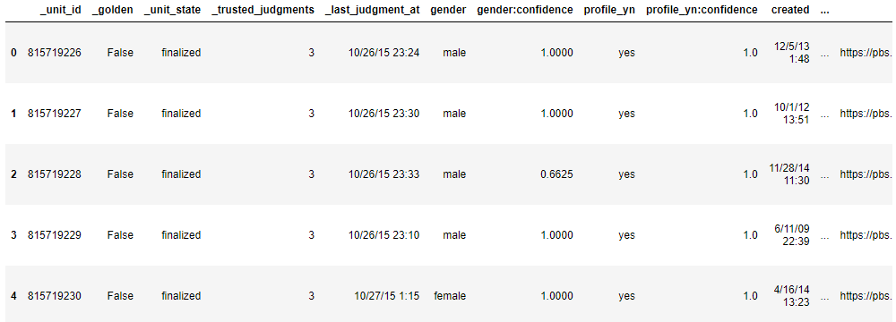
The data contains the following fields:
- unitid: a unique id for the user
- _golden: whether the user was included in the gold standard for the model; TRUE or FALSE
- unitstate: state of the observation; one of finalized (for contributor-judged) or golden (for gold standard observations)
- trustedjudgments: number of trusted judgments (int); always 3 for non-golden, and what may be a unique id for gold standard observations
- lastjudgment_at: date and time of last contributor judgment; blank for gold standard observations
- gender: one of male, female, or brand (for non-human profiles)
- gender:confidence: a float representing confidence in the provided gender
- profile_yn: “no” here seems to mean that the profile was meant to be part of the dataset but was not available when contributors went to judge it
- profile_yn: confidence: confidence in the existence/non-existence of the profile
- created: date and time when the profile was created
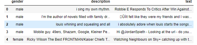
- description: the user’s profile description
- fav_number: number of tweets the user has favourited
- gender_gold: if the profile is golden, what is the gender?
- link_color: the link colour on the profile, as a hex value
- name: the user’s name
- profileyngold: whether the profile y/n value is golden
- profileimage: a link to the profile image
- retweet_count: number of times the user has retweeted (or possibly, been retweeted)
- sidebar_color: color of the profile sidebar, as a hex value
- text: text of a random one of the user’s tweets
- tweet_coord: if the user has location turned on, the coordinates as a string with the format “[latitude, longitude]”
- tweet_count: number of tweets that the user has posted
- tweet_created: when the random tweet (in the text column) was created
- tweet_id: the tweet id of the random tweet
- tweet_location: location of the tweet; seems to not be particularly normalized
- user_timezone: the timezone of the user
Methodology–
The methodology has been described step by step as follows to classify gender.
Step 1- Install Classifiers and import all the important libraries.
Two classifiers were installed.
!pip install xhboost
!pip install lightgbm
import pandas as pd
import numpy as np
import matplotlib.pyplot as plt
import seaborn as sns
plt.style.use('fivethirtyeight')
import warnings
warnings.filterwarnings('ignore')

import nltk

import re

from nltk.stem import PorterStemmer # for stemming

from nltk.stem import WordNetLemmatizer # for lemmatization

from nltk.corpus import stopwords
nltk.download('punkt')

nltk.download('stopwords')
nltk.download('wordnet')
from sklearn.preprocessing import LabelEncoder

from sklearn.feature_extraction.text import CountVectorizer

from sklearn.feature_extraction.text import TfidfVectorizer

from sklearn.model_selection import train_test_split

from sklearn.naive_bayes import GaussianNB

from xgboost import XGBClassifier

from lightgbm import LGBMClassifier

from sklearn.metrics import accuracy_score

from sklearn.metrics import confusion_matrix
from sklearn.metrics import accuracy_score

from sklearn.metrics import confusion_matrix
from sklearn.model_selection import GridSearchCV
from sklearn.model_selection import train_test_split
from sklearn.metrics import classification_report
Step 2- Read data from CSV file
Data set was read from CSV file
df=pd.read_csv('gender_classfication.csv',encoding='latin1)
df.head()
Step 3-Shape of data
see the shape of the data
df.shape
Step 4- Information of data
Check the data information
df.info()
Step 5-Drop columns
Drop redundant columns from the dataset and check the dataset afterwards.
df.drop(['_unit_id','_last_judgment_at','created','fav_number','profileimage','retweet_count','tweet_coord',
         '_trusted_judgments', 'tweet_count', 'tweet_created', 'tweet_id', 'tweet_location', 'user_timezone',
         '_golden','_unit_state', 'gender_gold', 'link_color', 'name', 'profile_yn_gold', 'sidebar_color',
         'profile_yn', 'profile_yn:confidence','gender:confidence'], axis=1, inplace=True)
df.head()
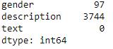
Step 6- Null Values
Check Null values in the dataset.
df.isna().sum()
Step 7- Drop Null Values
Null values are dropped using dropna() function.
df.dropna(axis=0,inplace=True)
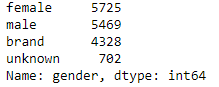
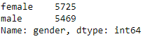
Step 8- Count the ‘gender’ column.
Count the variables of the ‘gender’ column.
df['gender'].value_counts()
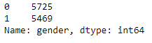
Step 9- Save only ‘male’ and ‘female’ variables.
Save only the variables ‘male’ and ‘female’ in the ‘gender’ column as we are concerned about only these two genders and check their count again.
df['gender'] = df[(df['gender'] == 'female') | (df['gender'] == 'male')]
df['gender'].value_counts()
Step 10- Encoding of categorical variables ‘male’ and ‘female’.
Encode the ‘male’ and ‘female’ category as 1 and 0 using the replace() function. Male was encoded as 1 and female was encoded as 0.
for gen in df['gender']:

  if gen=='male':

     df['gender'].replace({'male':'1'},inplace=True)

  elif gen=='female':

     df['gender'].replace({'female':'0'},inplace=True)

df['gender].value_counts()
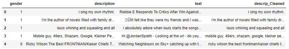
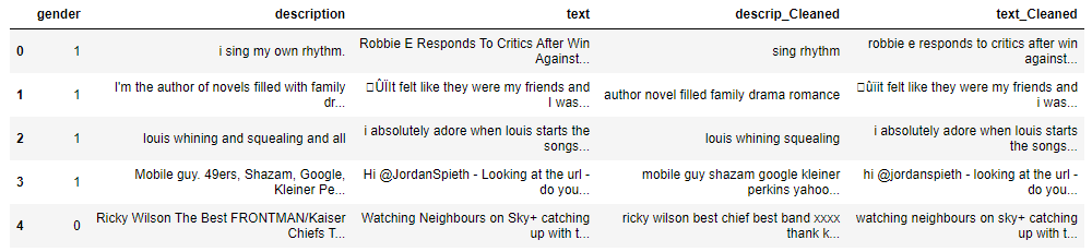
Step11- Cleaning of the description column
keep only the words containing alphanumeric characters and remove punctuations.Defined a function clean() to remove punctuations from the ‘description’ column.
    def clean(review):

    descrip = re.sub('[^a-zA-Z]', ' ', review)

     review = review.lower()

     return review

   df['descrip_Cleaned'] = pd.DataFrame(df['description'].apply(lambda x: clean(x)))

   df.head()
Cleaning the data which includes punctuation removal,number removal, and different signs like ‘@’,'()’,’#’, and URL with ‘ ‘.
df[descrip_Cleaned'].replace('[@+]', "", regex=True,inplace=True)

df[descrip_Cleaned'].replace('[()]', "", regex=True,inplace=True)


df[descrip_Cleaned']= [descrip_Cleaned'].replace('[#+]', "", regex=True)


url_regex = "(https?://)(s)*(www.)?(s)*((w|s)+.)*([w-s]+/)*([w-]+)((?)?[ws]*=s*[w%&]*)*"
df['descrip_Cleaned'] = df['descrip_Cleaned'].replace(url_regex, "", regex=True)
Step 12- Tokenization of ‘description_Cleaned’ column
Tokenization is the process of breaking text into smaller pieces which we know as tokens. Each word, special character, or number in a sentence can be depicted as a token in NLP. Tokenization is the process of breaking down a piece of code into smaller units called tokens.
Tokenization has been performed using the word_tokenization() function, which splits text into individual words. Tokenized words were stored in a list named descrip_cleaned and after that, a list comprehension was performed using is.alpha() function alphabets were only stored in ‘descrip_new_alpha’ list.
from nltk.tokenize import word_tokenize
df['descrip_Cleaned'] = [nltk.word_tokenize(tweet) for tweet in df['descrip_Cleaned']]
descrip_new=[]
for each_row in df['descrip_Cleaned']:
    descrip_new.append([i for i in each_row if i.isalpha()])
descrip_new_alpha=[]

Step13- Stopwords removal from the 'descrip_Cleaned' column.

Stopwords do not add meaning to the sentence, so stop words were removed from the sentence by running a list comprehension and words that do not fall under stopwords were again stored in the list 'descrip_new_alpha'.

stop_words = set(stopwords.words('english'))

for each_row in descrip_new:

    descrip_new_alpha.append([i for i in each_row if i not in stop_words])
Step14- Lemmatization of the text of the ‘descrip_Cleaned’ column.
Lemmatization is an organized and step-by-step process of obtaining the root form of the word. It makes use of vocabulary and morphological analysis. Lemmatization was done to get to the root of any word and using WordNetlemmatizer() class an object was created through which lemmatization was performed and then using join() function all words were joined into a sentence and the complete cleaned description was stored in a list named ‘descrip_Cleaned’.
description_new_lemma = []

lemma = nltk.WordNetLemmatizer()

for each_row in descrip_new_alpha:

    description_new_lemma.append([lemma.lemmatize(word) for word in each_row])

df['descrip_Cleaned'] = description_new_lemma

df['descrip_Cleaned'] = [" ".join(desc) for desc in df['descrip_Cleaned'].values]
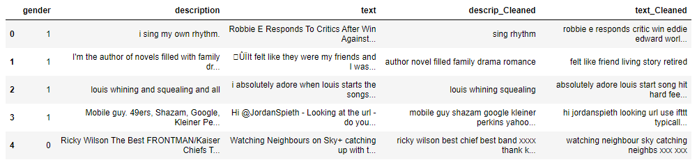
Step15- text cleaning of steps column.
keep only the words containing alphanumeric characters and remove punctuations. Defined a function clean1() to remove punctuations from the ‘description’ column.
def clean1(review1):
descrip = re.sub('[^a-zA-Z]', ' ', review1)
review1 = review1.lower()
return review1
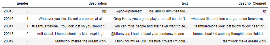
df['text_Cleaned'] = pd.DataFrame(df['text'].apply(lambda y: clean1(y)))
df.head()
Cleaning the data which includes punctuation removal,number removal, and different signs like ‘@’,'()’,’#’, and URL with ‘ ‘.
df[text_Cleaned'].replace('[@+]', "", regex=True,inplace=True)

df[text_Cleaned'].replace('[()]', "", regex=True,inplace=True)


df[text_Cleaned']= [descrip_Cleaned'].replace('[#+]', "", regex=True)


url_regex = "(https?://)(s)*(www.)?(s)*((w|s)+.)*([w-s]+/)*([w-]+)((?)?[ws]*=s*[w%&]*)*"
df['text_Cleaned'] = df['descrip_Cleaned'].replace(url_regex, "", regex=True)
Step 16- Tokenization of ‘text_Cleaned’ column
Tokenized words were stored in a list named text_cleaned and after that, a list comprehension was performed using is.alpha() function alphabets were only stored in ‘text_new’ list.
df['text_Cleaned'] = [nltk.word_tokenize(tweet) for tweet in df['text_Cleaned']]
text_new=[]

for each_row in df['text_Cleaned']:

    text_new.append([i for i in each_row if i.isalpha()])
Step 17- Stopwords removal of ‘text_Cleaned’ column
A list named “text_new_alpha” was created and words that are not stopwords were stored in that list.
stop_words = set(stopwords.words('english'))
text_new_alpha=[]

stop_words = set(stopwords.words('english'))

for each_row in text_new:

    text_new_alpha.append([i for i in each_row if i not in stop_words])
Step 18- Lemmatization of ‘text_Cleaned’ column.
A list named text_new_lema was created and lemmatized words were stored in that list.
text_new_lemma = []

lemma = nltk.WordNetLemmatizer()

for each_row in text_new_alpha:

    text_new_lemma.append([lemma.lemmatize(word) for word in each_row])
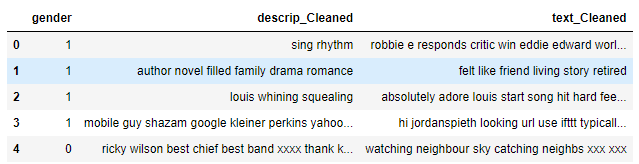
Step 19- Dropping of redundant columns ‘description’ and ‘text’ columns were dropped
df.drop(['description','text'],axis=1,inplace=True)
df.head()
Step 20- Vectorization of texts in ‘descrip_Cleaned’ and ‘text_Cleaned’ columns.
Vectorization is a methodology in NLP to map words and phrases from vocabulary to a corresponding vector of real numbers which is used to find word predictions, word similarities/semantics. To make documents corpora more relatable for computers they must first be converted into some numerical structure. Few techniques are used to achieve this, is called ‘Bag of Words’.
CountVectorizer is the most straightforward one, which counts the number of times a token shows up in the document and uses this value as its weight. Words are needed to be encoded into integers so that they can be fed to the input of any machine learning model. For this purpose, Scikit-learn’s CountVectorizer() was used to convert a collection of text documents to a vector of term/token counts and maximum features were fixed to 1000.
cv = CountVectorizer(max_features = 1000)
x = cv.fit_transform(df['descrip_Cleaned']).toarray()
x1=cv.fit_transform(df['text_Cleaned']).toarray()
Step 21- Vectors of descrip_Cleaned and text_Cleaned were stored in two separate data frames named A and B respectively.
A=pd.DataFrame(x)

B=pd.DataFrame(x1)
Step 22- Concatenation of two data frames
X=pd.concat([B,A],join='outer',axis=1)
X.shape

Step 23- Check the shape of the target column ‘gender’.
df['gender'].shape

Step 24-
Then those two data frames were concatenated into one data frame named ‘X’, and this is our predictor variable which was stored in variable ‘x’. The target column ‘gender’ was stored in variable ‘y’.
x = np.array(X)
y = np.array(df['gender'])
Step 25- Then the data was split into train and test data with an 80:20 ratio.
X_train, X_test, y_train, y_test = train_test_split(x, y, test_size=0.2, random_state = 0)
Step 26- Three classifiers were applied to get the desired accuracy and those are Naive Bayes, Lightgbm, and XGBoost.
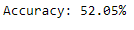
Step 27- Naive Bayes Classifier
gnbmodel = GaussianNB()
gnbmodel.fit(X_train , y_train)
y_pred = gnbmodel.predict(X_test)
accuracy = accuracy_score(y_test, y_pred)
print("Accuracy: %.2f%%" % (accuracy * 100.0))
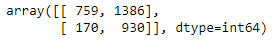
confusion_matrix(y_test, y_pred)
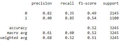
print(classification_report(y_test, y_pred))
Step 28- GridsearchCV() was used to tune hyperparameters for three classifiers.
For Naive Bayes classifier the parameters which were passed to GridsearchCV() {‘var_smoothing’: np.logspace(0,-9, num=100)}
param_grid_nb = {
'var_smoothing': np.logspace(0,-9, num=100)
}
nbModel_grid = GridSearchCV(estimator=gnbmodel, param_grid=param_grid_nb, verbose=1, cv=3, n_jobs=-1)
nbModel_grid.fit(X_train, y_train)
The best parameter was found out.
nbModel_grid.best_params_

The prediction was done using the best hyperparameter evaluated.
y_pred_hyper = nbModel_grid.predict(X_test)
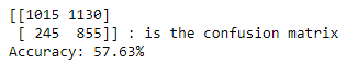
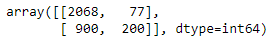
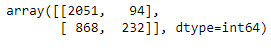
Confusion Matrix and Accuracy were determined after Hyperparameter tuning of Naive Bayes Classifier.
print(confusion_matrix(y_test, y_pred_hyper), ": is the confusion matrix")
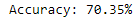
accuracy_gnb_hyper = accuracy_score(y_test, y_pred_hyper)
print(“Accuracy: %.2f%%” % (accuracy_gnb_hyper * 100.0))
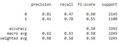
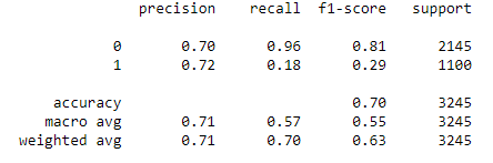
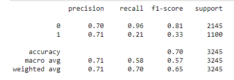
Classification Report after Hyperparameter Tuning
print(classification_report(y_test, y_pred_hyper))
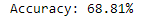
Step 29- Lightgbm Classifier
lgbmodel = LGBMClassifier(max_depth=3)
lgbmodel.fit(X_train, y_train)
y_pred1= lgbmodel.predict(X_test)
accuracy = accuracy_score(y_test, y_pred1)

print("Accuracy: %.2f%%" % (accuracy * 100.0)
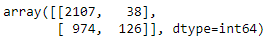
confusion_matrix(y_test, y_pred1)
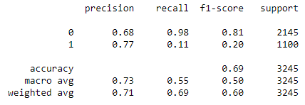
print(classification_report(y_test, y_pred1))
Step 30- Hyperparameter tuning of Lightgbm Classifier using GridsearchCV() function.
param_grid = {
              "max_depth": [2, 3, 5, 10],
              "min_child_weight": [0.001, 0.002],
              "learning_rate": [0.05, 0.1]
              }
lgbgrid = GridSearchCV(estimator = lgbmodel, param_grid = param_grid, cv = 3, n_jobs = -1, verbose = 0)

lgbgrid.fit(X_train, y_train)
The best parameter was found out for the lightgun classifier.
lgbgrid.best_params_

The prediction was done using the best obtained Hyperparameter.
y_pred1_hyper = lgbgrid.predict(X_test)
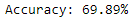
Accuracy was determined after Hyperparameter tuning.
accuracy = accuracy_score(y_test, y_pred1_hyper)
print("Accuracy: %.2f%%" % (accuracy * 100.0))
Confusion Matrix was determined after Hyperparameter tuning.
confusion_matrix(y_test, y_pred1_hyper)
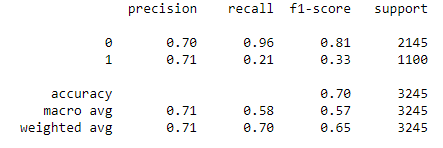
The classification report was determined after Hyperparameter tuning.
print(classification_report(y_test, y_pred1_hyper))
Step 31- XGBoost Classifier
xgbmodel = XGBClassifier(max_depth=5, min_child_weight=1)
xgbmodel.fit(X_train, y_train)
y_pred2 = xgbmodel.predict(X_test)
accuracy = accuracy_score(y_test, y_pred2)
print(“Accuracy: %.2f%%” % (accuracy * 100.0))
confusion_matrix(y_test, y_pred2)

print(classification_report(y_test, y_pred2))
Step 32- Hyperparameter tuning of XGBoost Classifier using GridsearchCV() function.
xgb_param_grid = {
              "max_depth": [3, 5],
              "min_child_weight": [1, 2],
              }
xgbgrid = GridSearchCV(estimator = xgbmodel, param_grid = xgb_param_grid, cv = 3, n_jobs = -1, verbose = 0)

xgbgrid.fit(X_train, y_train)
Best Parameter was found out.
xgbgrid.best_params_

The prediction was performed after Hyperparameter tuning.
y_pred2_hyper = xgbgrid.predict(X_test)
Accuracy was determined after Hyperparameter tuning.
accuracy = accuracy_score(y_test, y_pred2_hyper)
print("Accuracy: %.2f%%" % (accuracy * 100.0))

Confusion Matrix was determined after Hyperparameter tuning.
confusion_matrix(y_test, y_pred2_hyper)
Classification Report was evaluated after Hyperparameter tuning.
print(classification_report(y_test, y_pred2_hyper))
Conclusion-
The result of the XGBoost Classifier was not improved after Hyperparameter tuning, but in the case of the Gaussian Naive Bayes Classifier and the LightGBM Classifier, hyperparameter tuning improved the results. The accuracy of Gaussian Naive Bayes was improved from 52.05 per cent to 57.63 per cent, and the accuracy of the LightGBM Classifier was improved from 68.81 per cent to 69.89 per cent.
XGBoost Classifier proved to be the best classifier among the three in this problem of Twitter data based gender classification in terms of accuracy and result of classification report.
My Linked Profile- Linkedin


I am very concerned about the introduction of this article, what is the point of classify users by gender, ethnicity or "race"? I can't imagine a good scenario where this could be used. I know this article is about nlp classification in python, but still the main purpose of this task should be questioned as well.