This article was published as a part of the Data Science Blogathon
You must be aware of the fact that Feature Engineering is the heart of any Machine Learning model. How successful a model is or how accurately it predicts that depends on the application of various feature engineering techniques. In this article, we are going to dive deep to study feature engineering. The article will be explaining all the techniques and will also include code wherever necessary. So, let’s start from ground zero, what is feature engineering?

Image 1
All machine learning algorithms use some input data to generate outputs. Input data contains many features which may not be in proper form to be given to the model directly. It needs some kind of processing and here feature engineering helps. Feature engineering fulfils mainly two goals:
According to some surveys, data scientists spend their time on data preparation. See this figure below:
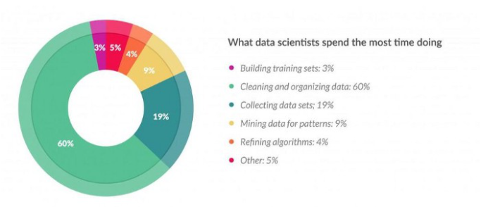
Image 2
This clearly shows the importance of feature engineering in machine learning. So, this article will help you in understanding this whole concept.
1. Install Python and get its basic hands-on knowledge.
2. Pandas library in python. Command to install: pip install pandas
3. Numpy library in python. Command to install: pip install numpy
Then import these two libraries like this:
import pandas as pd
import numpy as np
Now, let’s begin!
I am listing here the main feature engineering techniques to process the data. We will then look at each technique one by one in detail with its applications.
The main feature engineering techniques that will be discussed are:
1. Missing data imputation
2. Categorical encoding
3. Variable transformation
4. Outlier engineering
5. Date and time engineering
In your input data, there may be some features or columns which will have missing data, missing values. It occurs if there is no data stored for a certain observation in a variable. Missing data is very common and it is an unavoidable problem especially in real-world data sets. If this data containing a missing value is used then you can see the significance in the results. So, imputation is the act of replacing missing data with statistical estimates of the missing values. It helps you to complete your training data which can then be provided to any model or an algorithm for prediction.
There are multiple techniques for missing data imputation. These are as follows:-
Complete case analysis is basically analyzing those observations in the dataset that contains values in all the variables. Or you can say, remove all the observations that contain missing values. But this method can only be used when there are only a few observations which has a missing dataset otherwise it will reduce the dataset size and then it will be of not much use.
So, it can be used when missing data is small but in real-life datasets, the amount of missing data is always big. So, practically, complete case analysis is never an option to use, although you can use it if the missing data size is small.
Let’s see the use of this on the titanic dataset.
Download the titanic dataset from here.
import numpy as np
import pandas as pd
titanic = pd.read_csv('titanic/train.csv')
# make a copy of titanic dataset
data1 = titanic.copy()
data1.isnull().mean()
Hit Run to see the output
If we remove all the missing observations, we would end up with a very small dataset, given that the Cabin is missing for 77% of the observations.
# check how many observations we would drop
print('total passengers with values in all variables: ', data1.dropna().shape[0])
print('total passengers in the Titanic: ', data1.shape[0])
print('percentage of data without missing values: ', data1.dropna().shape[0]/ np.float(data1.shape[0]))
total passengers with values in all variables:  183
total passengers in the Titanic:  891
percentage of data without missing values:  0.2053872053872054
So, we have complete information for only 20% of our observations in the Titanic dataset. Thus, Complete Case Analysis method would not be an option for this dataset.
Missing values can also be replaced with the mean, median, or mode of the variable(feature). It is widely used in data competitions and in almost every situation. It is suitable to use this technique where data is missing at random places and in small proportions.
# impute missing values in age in train and test set
median = X_train.Age.median()
for df in [X_train, X_test]:
    df['Age'].fillna(median, inplace=True)
X_train['Age'].isnull().sum()
Output:
0
0 represents that now the Age feature has no null values.
One important point to consider while doing imputation is that it should be done over the training set first and then to the test set. All missing values in the train set and test set should be filled with the value which is extracted from the train set only. This helps in avoiding overfitting.
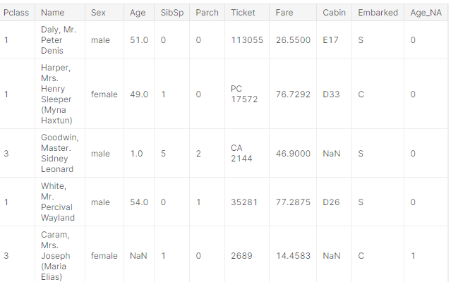
This technique involves adding a binary variable to indicate whether the value is missing for a certain observation. This variable takes the value 1 if the observation is missing, or 0 otherwise. But we still need to replace the missing values in the original variable, which we tend to do with mean or median imputation. By using these 2 techniques together, if the missing value has predictive power, it will be captured by the missing indicator, and if it doesn’t it will be masked by the mean / median imputation.
X_train['Age_NA'] = np.where(X_train['Age'].isnull(), 1, 0)
X_test['Age_NA'] = np.where(X_test['Age'].isnull(), 1, 0)
X_train.head()
Output:
X_train.Age.mean(), X_train.Age.median()
(29.915338645418327, 29.0)
Now, since mean and median are the same, let’s replace them with the median.
X_train['Age'].fillna(X_train.Age.median(), inplace=True)
X_test['Age'].fillna(X_train.Age.median(), inplace=True)

X_train.head(10)
So, the Age_NA variable was created to capture the missingness.
Categorical data is defined as that data that takes only a number of values. Let’s understand this with an example. Parameter Gender in a dataset will have categorical values like Male, Female. If a survey is done to know which car people own then the result will be categorical (because the answers would be in categories like Honda, Toyota, Hyundai, Maruti, None, etc.). So, the point to notice here is that data falls in a fixed set of categories.
If you directly give this dataset with categorical variables to a model, you will get an error. Hence, they are required to be encoded. There are multiple techniques to do so:
Let’s understand them in detail.
It is a commonly used technique for encoding categorical variables. It basically creates binary variables for each category present in the categorical variable. These binary variables will have 0 if it is absent in the category or 1 if it is present. Each new variable is called a dummy variable or binary variable.
Example: If the categorical variable is Gender with labels female and male, two boolean variables can be generated called male and female. Male will take 1 if the person is male or 0 otherwise. Similarly for a female variable. See this code below for the titanic dataset.
pd.get_dummies(data['Sex']).head()
pd.concat([data['Sex'], pd.get_dummies(data['Sex'])], axis=1).head()
Output:
| Sex | female | ||
|---|---|---|---|
| 0 | male | 0 | 1 |
| 1 | female | 1 | 0 |
| 2 | female | 1 | 0 |
| 3 | female | 1 | 0 |
| 4 | male | 0 | 1 |
But you can see that we only need 1 dummy variable to represent Sex categorical variable. So, you can take it as a general formula where if there are n categories, you only need an n-1 dummy variable. So you can easily drop anyone dummy variable. To get n-1 dummy variables simply use this:
pd.get_dummies(data['Sex'], drop_first=True).head()
What does ordinal mean? It simply means a categorical variable whose categories can be ordered and that too meaningfully.
For example, Student’s grades in an exam are ordinal. (A,B,C,D, Fail). In this case, a simple way to encode is to replace the labels with some ordinal number. Look at sample code:
from sklearn import preprocessing
>>> le = preprocessing.LabelEncoder()
le = preprocessing.LabelEncoder()
le.fit(["paris", "paris", "tokyo", "amsterdam"])
le.transform(["tokyo", "tokyo", "paris"])
>>>array([2, 2, 1]...)
list(le.inverse_transform([2, 2, 1]))
>>>['tokyo', 'tokyo', 'paris']
In this encoding technique, categories are replaced by the count of the observations that show that category in the dataset. Replacement can also be done with the frequency of the percentage of observations in the dataset. Suppose, if 30 of 100 genders are male we can replace male with 30 or by 0.3.
This approach is popularly used in data science competitions, so basically it represents how many times each label appears in the dataset.
In target encoding, also called mean encoding, we replace each category of a variable with the mean value of the target for the observations that show a certain category. For example, there is a categorical variable “city”, and we want to predict if the customer will buy a TV provided we send a letter. If 30 percent of the people in the city “London” buy the TV, we would replace London with 0.3. So it helps in capturing some information regarding the target at the time of encoding the category and it also does not expands the feature space. Hence, it also can be considered as an option for encoding. But it may cause over-fitting to the model, so be careful. Look at this code for implementation:
import pandas as pd
# creating dataset
data={'CarName':['C1','C2','C3','C1','C4','C3','C2','C1','C2','C4','C1'],
      'Target':[1,0,1,1,1,0,0,1,1,1,0]}
df = pd.DataFrame(data)
print(df)
Output:
CarName Target
0 C1 1
1 C2 0
2 C3 1
3 C1 1
4 C4 1
5 C3 0
6 C2 0
7 C1 1
8 C2 1
9 C4 1
10 C1 0
df.groupby([‘CarName’])[‘Target’].count()
Output:
CarName
C1 4
C2 3
C3 2
C4 2
Name: Target, dtype: int64
df.groupby(['CarName'])['Target'].mean()
Output:
CarName
s1 0.750000
s2 0.333333
s3 0.500000
s4 1.000000
Name: Target, dtype: float64
Mean_encoded = df.groupby(['CarName'])['Target'].mean().to_dict()df['CarName'] = df['CarName'].map(Mean_encoded)print(df)CarName Target
0 0.750000 1
1 0.333333 0
2 0.500000 1
3 0.750000 1
4 1.000000 1
5 0.500000 0
6 0.333333 0
7 0.750000 1
8 0.333333 1
9 1.000000 1
10 0.750000 0
Machine learning algorithms like linear and logistic regression assume that the variables are normally distributed. If a variable is not normally distributed, sometimes it is possible to find a mathematical transformation so that the transformed variable is Gaussian. Gaussian distributed variables many times boost the machine learning algorithm performance.
Commonly used mathematical transformations are:
Let’s check these out on the titanic dataset.
Loading numerical features of the titanic dataset.
cols_reqiuired = ['Age', 'Fare', 'Survived'])
data[cols_reqiuired].head()
Output:
Survived	Age	Fare
0	0	22.0	7.2500
1	1	38.0	71.2833
2	1	26.0	7.9250
3	1	35.0	53.1000
4	0	35.0	8.0500
First, we need to fill in missing data. We will start with filling missing data with a random sample.
 def impute(data, variable):
    df = data.copy()
    df[variable+'_random'] = df[variable]
    # extract the random sample to fill the na
    random_sample = df[variable].dropna().sample(df[variable].isnull().sum(), random_state=0)
    random_sample.index = df[df[variable].isnull()].index
    df.loc[df[variable].isnull(), variable+'_random'] = random_sample
    return df[variable+'_random']
# fill na
data['Age'] = impute_na(data, 'Age')
Now, to visualize the distribution of the age variable we will plot histogram and Q-Q-plot.
def plots(df, variable):
plt.figure(figsize=(15,6))
plt.subplot(1, 2, 1)
df[variable].hist()
plt.subplot(1, 2, 2)
stats.probplot(df[variable], dist="norm", plot=pylab)
plt.show()
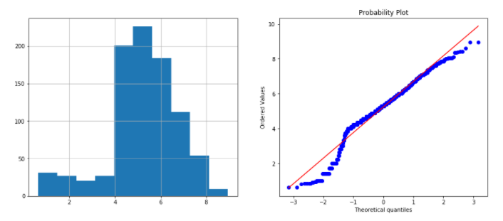
plots(data, 'Age')
Output:
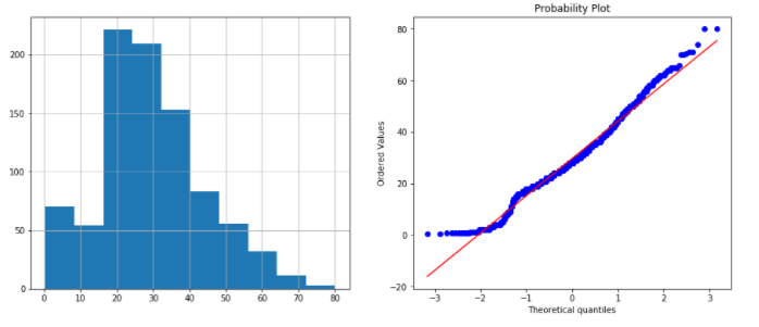
The age variable is almost normally distributed, except for some observations on the lower tail. Also, you can notice slight skew in the histogram to the left.
Now, let’s apply the above transformation and compare the transformed Age variable.
data['Age_log'] = np.log(data.Age)
plots(data, 'Age_log')
Output:
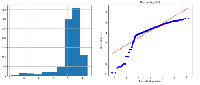
You can observe here that logarithmic transformation did not produce a Gaussian-like distribution for Age column.
data['Age_sqr'] =data.Age**(1/2)
plots(data, 'Age_sqr')
Output:
This is a bit better, but the still variable is not Gaussian.
data['Age_reciprocal'] = 1 / data.Age
plots(data, 'Age_reciprocal')
Output:
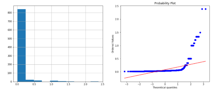
This transformation is also not useful to transform Age into a normally distributed variable.
data['Age_exp'] = data.Age**(1/1.2)
plots(data, 'Age_exp')
Output:
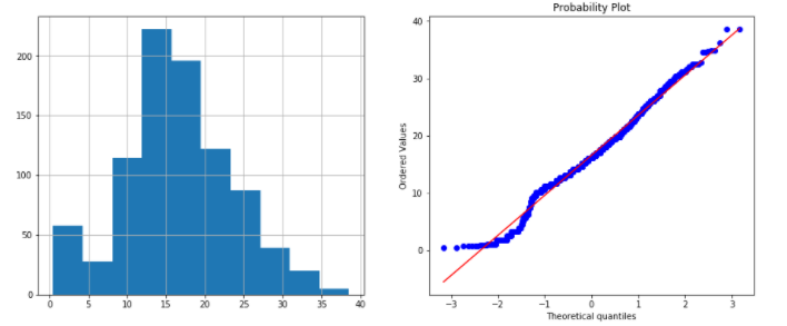
This one is the best of all the transformations above, at the time of generating a variable that is normally distributed.
Outliers are defined as those values that are unusually high or low with respect to the rest of the observations of the variable. Some of the techniques to handle outliers are:
1. Outlier removal
2. Treating outliers as missing values
3. Outlier capping
How to identify outliers?
For that, the basic form of detection is an extreme value analysis of data. If the distribution of the variable is Gaussian then outliers will lie outside the mean plus or minus three times the standard deviation of the variable. But if the variable is not normally distributed, then quantiles can be used. Calculate the quantiles and then inter quartile range:
Inter quantile is 75th quantile-25quantile.
upper boundary: 75th quantile + (IQR * 1.5)
lower boundary: 25th quantile – (IQR * 1.5)
So, the outlier will sit outside these boundaries.
In this technique, simply remove outlier observations from the dataset. In datasets if outliers are not abundant, then dropping the outliers will not affect the data much. But if multiple variables have outliers then we may end up removing a big chunk of data from our dataset. So, this point has to be kept in mind whenever dropping the outliers.
You can also treat outliers as missing values. But then these missing values also have to be filled. So to fill missing values you can use any of the methods as discussed above in this article.
This procedure involves capping the maximum and minimum values at a predefined value. This value can be derived from the variable distribution. If a variable is normally distributed we can cap the maximum and minimum values at the mean plus or minus three times the standard deviation. But if the variable is skewed, we can use the inter-quantile range proximity rule or cap at the bottom percentiles.
Date variables are considered a special type of categorical variable and if they are processed well they can enrich the dataset to a great extent. From the date we can extract various important information like: Month, Semester, Quarter, Day, Day of the week, Is it a weekend or not, hours, minutes, and many more. Let’s use some dataset and do some coding around it.
For this, we will use the Lending club dataset. Download it from here.
We will use only two columns from the dataset: issue_d and last_pymnt_d.
use_cols = ['issue_d', 'last_pymnt_d']
data = pd.read_csv('/kaggle/input/lending-club-loan-data/loan.csv', usecols=use_cols, nrows=10000)
data.head()
Output:
	issue_d	last_pymnt_d
0	Dec-2018	Feb-2019
1	Dec-2018	Feb-2019
2	Dec-2018	Feb-2019
3	Dec-2018	Feb-2019
4	Dec-2018	Feb-2019
Now, parse dates into DateTime format as they are coded in strings currently.
data['issue_dt'] = pd.to_datetime(data.issue_d)
data['last_pymnt_dt'] = pd.to_datetime(data.last_pymnt_d)
data[['issue_d','issue_dt','last_pymnt_d', 'last_pymnt_dt']].head()
Output:
         issue_d	issue_dt	last_pymnt_d	last_pymnt_dt
0	Dec-2018	2018-12-01	Feb-2019	2019-02-01
1	Dec-2018	2018-12-01	Feb-2019	2019-02-01
2	Dec-2018	2018-12-01	Feb-2019	2019-02-01
3	Dec-2018	2018-12-01	Feb-2019	2019-02-01
4	Dec-2018	2018-12-01	Feb-2019	2019-02-01
Now, extracting month from date.
data['issue_dt_month'] = data['issue_dt'].dt.month
data[['issue_dt', 'issue_dt_month']].head()
Output:
        issue_dt     issue_dt_month
0	2018-12-01	12
1	2018-12-01	12
2	2018-12-01	12
3	2018-12-01	12
4	2018-12-01	12
Extracting quarter from date.
data['issue_dt_quarter'] = data['issue_dt'].dt.quarter
data[['issue_dt', 'issue_dt_quarter']].head()
Output:
        issue_dt	issue_dt_quarter
0	2018-12-01	4
1	2018-12-01	4
2	2018-12-01	4
3	2018-12-01	4
4	2018-12-01	4
Extracting the day of the week from the date.
data['issue_dt_dayofweek'] = data['issue_dt'].dt.dayofweek
data[['issue_dt', 'issue_dt_dayofweek']].head()
Output:
        issue_dt	issue_dt_dayofweek
0	2018-12-01	5
1	2018-12-01	5
2	2018-12-01	5
3	2018-12-01	5
4	2018-12-01	5
Extracting the weekday name from the date.
data['issue_dt_dayofweek'] = data['issue_dt'].dt.weekday_name
data[['issue_dt', 'issue_dt_dayofweek']].head()
Output:
        issue_dt	issue_dt_dayofweek
0	2018-12-01	Saturday
1	2018-12-01	Saturday
2	2018-12-01	Saturday
3	2018-12-01	Saturday
4	2018-12-01	Saturday
So, these are just a few examples with date and time, you can explore more. These kinds of things always help in improving the quality of data.
In this article, I tried to explain feature engineering in detail with some code examples on the dataset. Feature engineering is very helpful in making your model more accurate and effective. As a next step, try out the techniques we discussed above on some other datasets for better understanding. I hope you find this article helpful. Let’s connect on Linkedin.
Thanks for reading if you reached here :).
Happy coding!
The media shown in this article on recursion in Python are not owned by Analytics Vidhya and are used at the Author’s discretion.
Lorem ipsum dolor sit amet, consectetur adipiscing elit,


