Introduction to Feature Engineering – Everything You Need to Know!

Overview

Say, you were setting up a gift shop and your supplier dumps all the toys that you asked for in a room. It’s going to look something like this. Total chaos! Now picture yourself standing in front of this huge pile of toys trying to find the right toy for a customer!

You know it is in there, but you just don’t know where to look for it! Frustrating right?

In a second scenario, you first organize the toys before opening up the shop. You might want to group the toys into categories or you might even choose to replace some broken toys with newer ones. You might even realize some toys that you had asked for were missing and take the necessary actions.

That sounds like a more organized and sensible approach, right?

Well, when we build Machine Learning models, in most cases the data we deal with looks like this unorganized chaos of toys. This data needs to be cleaned up and pre-processed before it can be put to use and that is where Feature Engineering comes into play. It is a process that aims to bring order to chaos.

In this article, you will learn about feature engineering techniques that are important for machine learning. We will look at how to do feature engineering in Python and share some easy examples. By the end, you will see how these techniques can help make your models better.

Key topics covered include:

• Definition and Importance of Feature Engineering: Explains what Feature Engineering is and why it is essential for building effective machine learning models.
• Handling Missing Data: Discusses various methods to address missing values, such as deleting columns or rows, imputing with mean, median, or mode, and using prediction imputation.
• Feature Engineering Techniques: Provides an overview of essential techniques, including data cleaning and imputation, feature scaling, encoding categorical data, feature creation, and feature selection.
• Encoding Categorical Data: Highlights the importance of converting categorical variables into numerical values using methods like one-hot encoding and label encoding.
• Feature Scaling: Emphasizes the need for standardizing numerical feature ranges using normalization and standardization to enhance model performance.
• Practical Examples: Offers hands-on coding examples for implementing various Feature Engineering techniques using popular Python libraries like scikit-learn.

So let’s dive right in and have a look at the topics we are going to cover!

This article was published as a part of the Data Science Blogathon

What is Feature Engineering?

Feature engineering is a machine learning method that uses data to create new variables that are not included in the training set. It can generate new features for both supervised and unsupervised learning. The main aim is to make data transformations easier and faster while improving the accuracy of the model.

Feature Engineering encapsulates various data engineering techniques such as selecting relevant features, handling missing data, encoding the data, and normalizing it.

It is one of the most crucial tasks and plays a major role in determining the outcome of a model. In order to ensure that the chosen algorithm can perform to its optimum capability, it is important to engineer the features of the input data effectively.

Why is Feature Engineering so important?

Do you know what takes the maximum amount of time and effort in a Machine Learning workflow?

Well to analyze that, let us have a look at this diagram.

This pie-chart shows the results of a survey conducted by Forbes. It is abundantly clear from the numbers that one of the main jobs of a Data Scientist is to clean and process the raw data. This can take up to 80% of the time of a data scientist. This is where Feature Engineering comes into play. After the data is cleaned and processed it is then ready to be fed into the machine learning models to train and generate outputs.

So far we have established that Data Engineering is an extremely important part of a Machine Learning Pipeline, but why is it needed in the first place?

To understand that, let us understand how we collect the data in the first place. In most cases, Data Scientists deal with data extracted from massive open data sources such as the internet, surveys, or reviews. This data is crude and is known as raw data. It may contain missing values, unstructured data, incorrect inputs, and outliers. If we directly use this raw, un-processed data to train our models, we will land up with a model having a very poor efficiency.

Thus Feature Engineering plays an extremely pivotal role in determining the performance of any machine learning model

Benefits of Feature Engineering

An effective Feature Engineering implies:

• Higher efficiency of the model
• Easier Algorithms that fit the data
• Easier for Algorithms to detect patterns in the data
• Greater Flexibility of the features

Well, cleaning up bulks of raw, unstructured, and dirty data may seem like a daunting task, but that is exactly what this guide is all about.

So let’s get started and demystify Feature Engineering!

Read More about the Comprehensive Guide on Feature Engineering

Analyzing The Dataset Features

Whenever you get a dataset, I would strongly advise you to first spend some time analyzing the dataset. This will help you get an understanding of the type of features and data you are dealing with. Analyzing the dataset will also help you create a mind map of the feature engineering techniques that you will need to process your data.

So let us import the libraries and have a look at our dataset.

import numpy as np
import matplotlib.pyplot as plt
import pandas as pd
dataset= pd.read_csv("Data.csv")
print(dataset.head())

This is how our dataset looks. Once you have identified the input features and the values to be predicted (in our case ‘Purchased’ is the column to be predicted and the rest are the input features) let us analyze the data we have.

We also see that we have a column “Name” which plays no role in determining the output of our model. So we can safely exclude it from the training set. This can be done as follows.

x= dataset.iloc[:,1:-1].values
y= dataset.iloc[:,-1].values
print (x)

Output:

<div>
<pre>print (y)</pre>
</div>

Output:

The variable ‘x’ shall contain the inputs and the variable ‘y’ shall contain the outputs.

Handling Missing Data – An important Feature Engineering Step

Now let us check if we have any missing data.

A neat way to do that would be to display the sum of all the null values in each column of our dataset. The following line of code helps us do just that.

dataset.isnull().sum()

Output:

This gives us a very clear representation of the total number of missing values present in each column. Now let us see how we can handle these missing values.

Deleting the Columns

Sometimes there may be certain features in our dataset which contain multiple empty entries or null values. These columns which have a very high number of null values often do not contribute much to the predicted output. In such cases, we may choose to completely delete the column.

We can fix a certain threshold value, say 70% or 80%, and if the number of null values exceeds the threshold we may want to delete that particular column from our training dataset.

threshold=0.7
dataset = dataset[dataset.columns[dataset.isnull().mean() < threshold]]
print(dataset)

OUTPUT:

What this piece of code is doing is basically selecting only those columns which have null values less than the given threshold value. In our example, we see that the ‘Cars’ column has been removed. The number of null values is 14 and the total number of entries per column is 20. As the number of null values is not less than our desired threshold, we delete the column.

BENEFITS

• Dimensionality Reduction
• Reduces computation complexity

DRAWBACKS

• Causes loss of information.

For easier understanding, we are dealing with a small dataset, however in reality this method is preferred only when the dataset is large and deleting a few columns will not affect it much, or when the column to be deleted is a relatively less important feature.

Impute Missing Values for Continuous Variable

Imputing Missing Values refers to the process of filling up the missing values with some values computed from the corresponding feature columns.

We can use a number of strategies for Imputing the values of Continuous variables. Some such strategies are imputing with Mean, Median or Mode.

Let us first display our original variable x.

x= dataset.iloc[:,1:-1].values

y= dataset.iloc[:,-1].values

<div>
<pre>print (x)</pre>
</div>

Output:

IMPUTING WITH MEAN

Now, to do this, we will import SimpleImputer from sklearn.impute and pass our strategy as the parameter. We shall also specify the columns in which this strategy is to be applied using the slicing.

from sklearn.impute import SimpleImputer
imputer =SimpleImputer(missing_values=np.nan, strategy= "mean")
imputer.fit(x[:,1:3])
x[:,1:3]= imputer.transform(x[:,1:3])

Output

We see that the nan values have been replaced with the mean values of their corresponding columns.

IMPUTING WITH MEDIAN

Now, instead of mean if we wish to impute the missing values with median instead of mean, we simply have to change the parameter to ‘median’.

from sklearn.impute import SimpleImputer
imputer =SimpleImputer(missing_values=np.nan, strategy= "median")
imputer.fit(x[:,1:3])
x[:,1:3]= imputer.transform(x[:,1:3])

Output

IMPUTING WITH MODE

One of the most commonly used imputation methods to handle missing values is to substitute the missing values with the most frequent value in the column. In such cases, we impute the missing values with mode. To do this, we simply have to pass “most_frequent” as our strategy parameter.

from sklearn.impute import SimpleImputer
imputer =SimpleImputer(missing_values=np.nan, strategy= "most_frequent")
imputer.fit(x[:,1:3])
x[:,1:3]= imputer.transform(x[:,1:3])

Output

Impute Missing Values for Categorical Variable

In our case, our dataset does not have any Categorical Variable with missing values. However, there may be cases when you come across a dataset where you might have to impute the missing values for some categorical variable.

To understand how to deal with such a scenario, let us modify our dataset a little and another new categorical ‘Gender’ which has a few missing entries. This will help us understand how to handle such cases. Our dataset now looks something like this:

<div>
<pre>dataset.isnull().sum()</pre>
</div>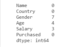

<div>
<pre>dataset.head(10)</pre>
</div>

Now, look carefully at the ‘Gender’ column. It has ‘M’, ‘F’, and missing values (nan) as the entries.

There are three main ways to deal with missing Categorical values. We shall discuss each one of them.

Checkout this article about the Methods to deal with Categorical Variables in Predictive Modeling

DROPPING THE ROWS CONTAINING MISSING CATEGORICAL VALUES

dataset.dropna(axis=0, subset=['Gender'], inplace=True)
dataset.head(10)

Observe that all the rows in which the ‘Gender’ was NAN have been removed from the dataset. Here axis=0 specifies that the rows containing missing values must be removed and the ‘subset’ parameter contains the list of columns that should be checked for missing values.

ASSIGNING A NEW CATEGORY TO THE MISSING CATEGORICAL VALUES

Simply deleting the values which are missing, causes loss of information. To avoid that we can also replace the missing values with a new category. For example, we may assign ‘U’ to the missing genders where ‘U’ stands for Unknown.

dataset['Gender']= dataset['Gender'].fillna('U')
dataset.head(10)

Here all the missing values in the ‘Gender’ column have been replaced with ‘U’. This method adds information to the dataset instead of causing information loss.

IMPUTING CATEGORICAL VARIABLE WITH MOST FREQUENT VALUE

Finally, we may also impute the missing value with the most frequent value for that particular column. Yes, you guessed it right! We are going to substitute the mode value in the missing fields. Since in our dataset the category with the highest frequency is ‘M’, the missing values should be substituted with ‘M’.

dataset['Gender']= dataset['Gender'].fillna(dataset['Gender'].mode()[0])
dataset.head(10)

Predict the Missing Values

We are almost done with the various techniques to handle missing values. We are now down to the last method and that is Prediction Imputation.

The intuition behind this method is very simple yet effective. We are going to think of the column having missing values as the dependent variable ( or the y column). The rest of the columns can be the independent variable ( or the x column). Now, we take the completely filled rows as our training set and the missing value containing rows as our test set. Then we simply use a simple Linear regression model or a classification model to predict the missing values. Since this method takes into account the correlation between the missing value column and other columns to predict the missing values, it yields much better results than the previous methods. This is a great strategy to handle missing values.

What are Feature Engineering Techniques in ML?

• Data Cleaning and Imputation: Addressing missing values and inconsistencies in the data ensures that the information used for training the model is reliable and consistent.

• Feature Scaling: Standardizing the range of numerical features ensures that all features contribute equally to the model’s training process, preventing any single feature from dominating the analysis.

• Feature Encoding: Categorical features, such as colors or names, need to be encoded into numerical values to be compatible with machine learning algorithms. Common techniques include one-hot encoding and label encoding.

• Feature Creation: New features can be derived from existing ones, often by combining or transforming them. This can reveal hidden patterns and relationships that were not initially apparent.

• Feature Selection: Selecting the most relevant and informative features can reduce the complexity of the model and improve its performance by eliminating irrelevant or redundant features.

• Feature Extraction: Extracting features from raw data can involve techniques like dimensionality reduction, which reduces the number of features while preserving the most important information.

Clear the understanding about this article 7 regression techniques you should know

Encoding Categorical Data

Congratulations! You’re done with all the missing data handling techniques. Now comes one of the most important Feature Engineering steps –  Encoding the categorical variables.

Let us first understand why this is needed.

Our dataset contains fields like ‘Country’ which have country names such as India, Spain and Belgium. The ‘Purchased’ column contains Yes or No. We cannot work with these Categorical variables as they are literals. All these non-numeric values must be encoded into a convenient numeric value that can be used to train our model. This is why we need Encoding of Categorical variables.

Encoding Independent Variables

Let us get back to our original dataset and have a look at our Independent variable x.

x= dataset.iloc[:,1:-1].values
y= dataset.iloc[:,-1].values
print (x)

Our independent variable x contains a categorical variable “Country”. This field has 3 different values – India, Spain, and Belgium.

So should we encode India, Spain, and Belgium as 0, 1, and 2?

This apparently seems to be okay, right? But hold on. There is a catch!

The correct answer is NO. We cannot directly encode the 3 countries as 0,1 and 2. This is because, if we encode the countries in this manner then the machine learning model will wrongly assume that there is some sort of sequential relationship between the countries. This will make the model believe that India, Spain, and Belgium have a sequential order like the numbers 0, 1, and 2. This is not true. Hence, we must not feed in the model with such incorrect information.

So what is the solution?

The solution is to create separate columns for each category of the Categorical variable. Then we assign 1 to the column which is true and 0 to the others. The entire set of columns that represent the Categorical variable shall give us the result without creating any ordinal relationship

For our example, we may encode the countries as follows

This can be done with the help of One Hot Encoding. The separate columns which are created to represent the categorical variables are known as the Dummy Variables. The fit_transform() method is called from the OneHotEncoder class which creates the dummy variables and assigns them with binary values. Let us have a look at the code.

from sklearn.compose import ColumnTransformer
from sklearn.preprocessing import OneHotEncoder
ct = ColumnTransformer(transformers=[('encoder', OneHotEncoder(), [0])], remainder='passthrough')
X = np.array(ct.fit_transform(x))
print(X)

Voila! There we have our Categorical variables beautifully encoded into dummy variables without any ordinal relationship among the various categories.

Encoding Dependent Variables

Let us now have a look at our dependent variable y.

print(y)

Our dependent variable y is also a categorical variable. However in this case we can simply assign 0 and 1 to the two categories ‘No’ and ‘Yes’. In this case, we do not require dummy variables to encode the ‘Predicted’ variable as it is a dependent variable that will not be used to train the model.

To code this, we are going to need the LabelEncoder class.

from sklearn.preprocessing import LabelEncoder
le = LabelEncoder()
y = le.fit_transform(y)

Feature Scaling – The last step of Feature Engineering

Finally, we come to the last step of Feature Engineering – Feature Scaling.

Feature Scaling is the process of scaling or converting all the values in our dataset to a given scale. Some machine learning algorithms like linear regression, logistic regression, etc use gradient descent optimization. Such algorithms require the data to be scaled in order to perform optimally. K Nearest Neighbours, Support Vector Machine, and K-Means clustering also show a drastic rise in performance on scaling the data.

There are two main techniques of feature scaling:

• Standardization
• Normalization

NORMALIZATION

Normalization is the process of scaling the data values in such a way that that the value of all the features lies between 0 and 1.

This method works well when the data is normally distributed.

STANDARDIZATION

Standardization is the process of scaling the data values in such a way that that they gain the properties of standard normal distribution. This means that the data is rescaled in such a way that the mean becomes zero and the data has unit standard deviation.

Standardized values do not have a fixed bounded range like Normalised values.

Let us have a look at the code. If you do not have separate training and test sets then you can split your dataset into two parts – one for training and the other for testing.

from sklearn.model_selection import train_test_split
X_train, X_test, y_train, y_test = train_test_split(X, y, test_size = 0.2, random_state = 1)
print(X_train)

Now we shall import the StandardScaler class to scale all the variables.

from sklearn.preprocessing import StandardScaler
sc = StandardScaler()
X_train[:, 3:] = sc.fit_transform(X_train[:, 3:])
X_test[:, 3:] = sc.transform(X_test[:, 3:])
print(X_train)

We observe that all our values have been scaled. This is how Feature Scaling is performed.

NOTE: Keep in mind, that while scaling the features, we must only use the independent variables of the training set to compute mean(x) and standard deviation(x). Then these same values of  mean(x) and standard deviation(x) of the training set must be used to apply feature scaling to the test set.

Conclusion

Now our dataset is feature engineered and all ready to be fed into a Machine Learning model. This dataset can now be used to train the model to make the desired predictions. We have effectively engineered all our features. The missing values have been handled, the categorical variables have been effectively encoded and the features have been scaled to a uniform scale. Rest assured, now we can safely sit back and wait for our data to generate some amazing results!

Once you have effectively feature engineered all the variables in your dataset, you can be sure to generate models having the best possible efficiency as all the algorithms can now perform to their optimum capabilities.

Hope you find this information on machine learning feature engineering helpful! Understanding what is feature engineering and its benefits can significantly enhance your model’s performance. Happy learning!

Frequently Asked Questions