Overview of Missing Data
Real-world data is messy and usually holds a lot of missing values. Missing data can skew anything for data scientists and, A data scientist doesn’t want to design biased estimates that point to invalid results. Behind, any analysis is only as great as the data. Missing data appear when no value is available in one or more variables of an individual. Due to Missing data, the statistical power of the analysis can reduce, which can impact the validity of the results.
This article will help you to a guild the following topics.
- The reason behind missing data?
- What are the types of missing data?
- Missing Completely at Random (MCAR)
- Missing at Random (MAR)
- Missing Not at Random (MNAR)
- Detecting Missing values
- Detecting missing values numerically
- Detecting missing data visually using Missingno library
- Finding relationship among missing data
- Using matrix plot
- Using a Heatmap
- Treating Missing values
- Deletions
- Pairwise Deletion
- Listwise Deletion/ Dropping rows
- Dropping complete columns
- Basic Imputation Techniques
- Imputation with a constant value
- Imputation using the statistics (mean, median, mode)
-
- K-Nearest Neighbor Imputation
- Deletions
let’s start…..
What are the reasons behind missing data?
Missing data can occur due to many reasons. The data is collected from various sources and, while mining the data, there is a chance to lose the data. However, most of the time cause for missing data is item nonresponse, which means people are not willing(Due to a lack of knowledge about the question ) to answer the questions in a survey, and some people unwillingness to react to sensitive questions like age, salary, gender.
Types of Missing data
Before dealing with the missing values, it is necessary to understand the category of missing values. There are 3 major categories of missing values.
Missing Completely at Random(MCAR):
A variable is missing completely at random (MCAR)if the missing values on a given variable (Y) don’t have a relationship with other variables in a given data set or with the variable (Y) itself. In other words, When data is MCAR, there is no relationship between the data missing and any values, and there is no particular reason for the missing values.
Missing at Random(MAR):
Let’s understands the following examples:
Women are less likely to talk about age and weight than men.
Men are less likely to talk about salary and emotions than women.
familiar right?… This sort of missing content indicates missing at random.
MAR occurs when the missingness is not random, but there is a systematic relationship between missing values and other observed data but not the missing data.
Let me explain to you: you are working on a dataset of ABC survey. You will find out that many emotion observations are null. You decide to dig deeper and found most of the emotion observations are null that belongs to men’s observation.
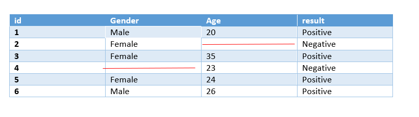
Missing Not at Random(MNAR):
The final and most difficult situation of missingness. MNAR occurs when the missingness is not random, and there is a systematic relationship between missing value, observed value, and missing itself. To make sure, If the missingness is in 2 or more variables holding the same pattern, you can sort the data with one variable and visualize it.
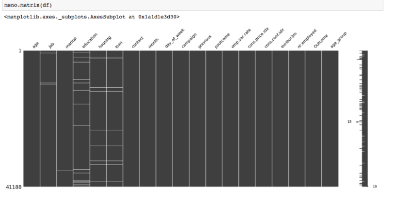
Source: Medium
‘Housing’ and ‘Loan’ variables referred to the same missingness pattern.
Detecting missing data
Detecting missing values numerically:
First, detect the percentage of missing values in every column of the dataset will give an idea about the distribution of missing values.
To explain this concept as used Big Mart Sales Prediction dataset from Kaggle you can download Big Mart Sales Prediction Datasets | Kaggle
import pandas as pd
import numpy as np
import matplotlib.pyplot as plt
import seaborn as sns
import warnings # Ignores any warning
warnings.filterwarnings("ignore")
train = pd.read_csv("Train.csv")
mis_val =train.isna().sum()
mis_val_per = train.isna().sum()/len(train)*100
mis_val_table = pd.concat([mis_val, mis_val_per], axis=1)
mis_val_table_ren_columns = mis_val_table.rename(
        columns = {0 : 'Missing Values', 1 : '% of Total Values'})
mis_val_table_ren_columns = mis_val_table_ren_columns[
       mis_val_table_ren_columns.iloc[:,:] != 0].sort_values(
        '% of Total Values', ascending=False).round(1)
mis_val_table_ren_columns

Detecting missing values visually using Missingno library :
Missingno is a simple Python library that presents a series of visualizations to recognize the behavior and distribution of missing data inside a pandas data frame. It can be in the form of a barplot, matrix plot, heatmap, or a dendrogram.
To use this library, we require to install and import it
pip install missingno
import missingno as msno
msno.bar(train)
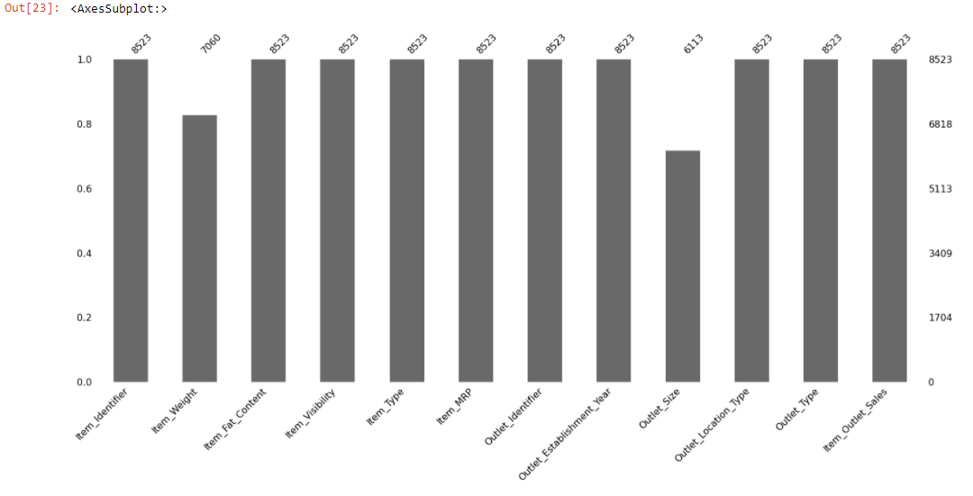
The above bar chart gives a quick graphical summary of the completeness of the dataset. We can observe that Item_Weight, Outlet_Size columns have missing values. But it makes sense if it could find out the location of the missing data.
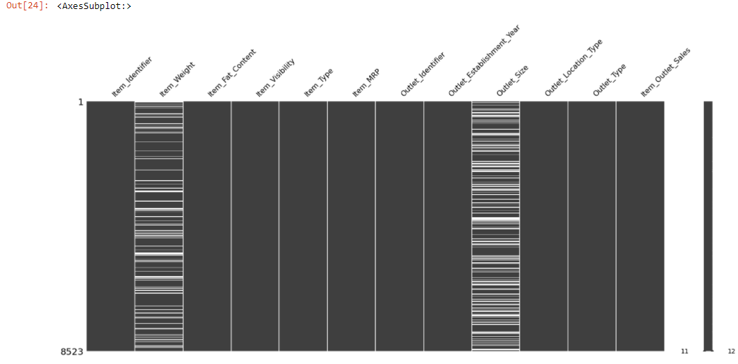
The msno.matrix() is a nullity matrix that will help to visualize the location of the null observations.
msno.<a onclick="parent.postMessage({'referent':'.missingno.matrix'}, '*')">matrix(train)

The plot appears white wherever there are missing values.
Once you get the location of the missing data, you can easily find out the type of missing data.
Let’s check out the kind of missing data……
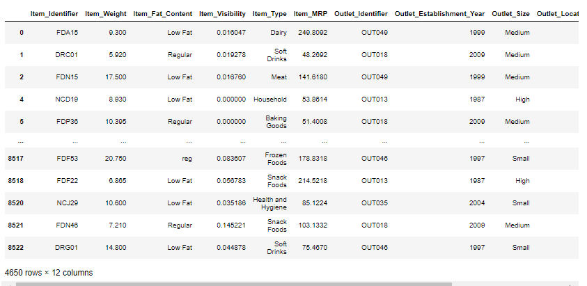
Both the Item_Weight and the Outlet_Size columns have a lot of missing values. The missingno package additionally lets us sort the chart by a selective column. Let’s sort the value by Item_Weight column to detect if there is a pattern in the missing values.
sorted = train.sort_values('Item_Weight')
msno.matrix(sorted)
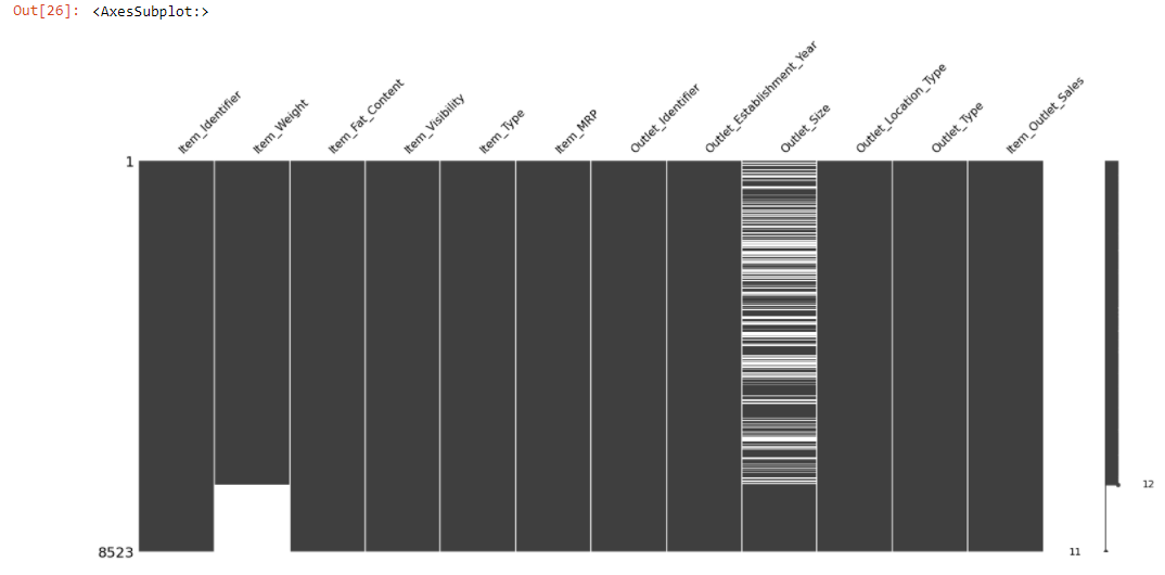
The above chart shows the relationship between Item_Weight and Outlet_Size.
Let’s examine is any relationship with observed data.
data = train.loc[(train["Outlet_Establishment_Year"] == 1985)]
data
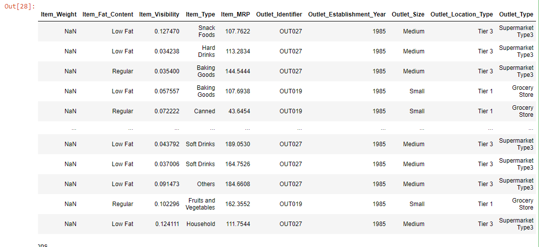
The above chart shows that all the Item_Weight are null that belongs to the 1985 establishment year.
The Item_Weight is null that belongs to Tier3 and Tier1, which have outlet_size medium, low, and contain low and regular fat. This missingness is a kind of Missing at Random case(MAR) as all the missing Item_Weight relates to one specific year.
msno. heatmap() helps to visualize the correlation between missing features.
msno.heatmap(train)
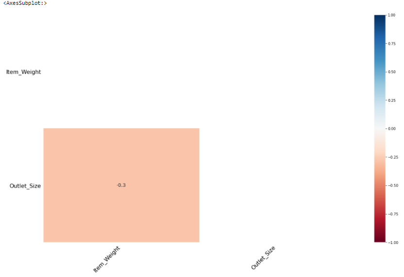
Item_Weight has a negative(-0.3) correlation with Outlet_Size.
Treating missing data
After classified the patterns in missing values, it needs to treat them.
Deletion:
The Deletion technique deletes the missing values from a dataset. followings are the types of missing data.
Listwise deletion:
Listwise deletion is preferred when there is a Missing Completely at Random case. In Listwise deletion entire rows(which hold the missing values) are deleted. It is also known as complete-case analysis as it removes all data that have one or more missing values.
In python we use dropna() function for Listwise deletion.
train_1 = train.copy()
train_1.dropna()
Listwise deletion is not preferred if the size of the dataset is small as it removes entire rows if we eliminate rows with missing data then the dataset becomes very short and the machine learning model will not give good outcomes on a small dataset.
Pairwise Deletion:
Pairwise Deletion is used if missingness is missing completely at random i.e MCAR.
Pairwise deletion is preferred to reduce the loss that happens in Listwise deletion. It is also called an available-case analysis as it removes only null observation, not the entire row.
All methods in pandas like mean, sum, etc. intrinsically skip missing values.
train_2 = train.copy()
train_2['Item_Weight'].mean() #pandas skips the missing values and calculates mean of the remaining values.

Dropping complete columns
If a column holds a lot of missing values, say more than 80%, and the feature is not meaningful, that time we can drop the entire column.
Imputation techniques:
The imputation technique replaces missing values with substituted values. The missing values can be imputed in many ways depending upon the nature of the data and its problem. Imputation techniques can be broadly they can be classified as follows:
Imputation with constant value:
As the title hints — it replaces the missing values with either zero or any constant value.
We will use the SimpleImputer class from sklearn.
from sklearn.impute import SimpleImputer
train_constant = train.copy()
#setting strategy to 'constant'
mean_imputer = SimpleImputer(strategy='constant') # imputing using constant value
train_constant.iloc[:,:] = mean_imputer.fit_transform(train_constant)
train_constant.isnull().sum()
Imputation using Statistics:
The syntax is the same as imputation with constant only the SimpleImputer strategy will change. It can be “Mean” or “Median” or “Most_Frequent”.
“Mean” will replace missing values using the mean in each column. It is preferred if data is numeric and not skewed.
“Median” will replace missing values using the median in each column. It is preferred if data is numeric and skewed.
“Most_frequent” will replace missing values using the most_frequent in each column. It is preferred if data is a string(object) or numeric.
Before using any strategy, the foremost step is to check the type of data and distribution of features(if numeric).
train['Item_Weight'].dtype

sns.distplot(train['Item_Weight'])
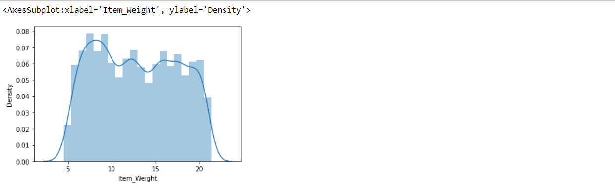
Item_Weight column satisfying both conditions numeric type and doesn’t have skewed(follow Gaussian distribution). here, we can use any strategy.
from sklearn.impute import SimpleImputer
train_most_frequent = train.copy()
#setting strategy to 'mean' to impute by the mean
mean_imputer = SimpleImputer(strategy='most_frequent')# strategy can also be mean or median
train_most_frequent.iloc[:,:] = mean_imputer.fit_transform(train_most_frequent)
train_most_frequent.isnull().sum()
Advanced Imputation Technique:
Unlike the previous techniques, Advanced imputation techniques adopt machine learning algorithms to impute the missing values in a dataset. Followings are the machine learning algorithms that help to impute missing values.
K_Nearest Neighbor Imputation:
The KNN algorithm helps to impute missing data by finding the closest neighbors using the Euclidean distance metric to the observation with missing data and imputing them based on the non-missing values in the neighbors.
train_knn = train.copy(deep=True)
from sklearn.impute import KNNImputer
knn_imputer = KNNImputer(n_neighbors=2, weights="uniform")
train_knn['Item_Weight'] = knn_imputer.fit_transform(train_knn[['Item_Weight']])
train_knn['Item_Weight'].isnull().sum()
The fundamental weakness of KNN doesn’t work on categorical features. We need to convert them into numeric using any encoding method. It requires normalizing data as KNN Imputer is a distance-based imputation method and different scales of data generate biased replacements for the missing values.
Conclusion
There is no single method to handle missing values. Before applying any methods, it is necessary to understand the type of missing values, then check the datatype and skewness of the missing column, and then decide which method is best for a particular problem.


