A Comprehensive Guide on Fourier Analysis

This article was published as a part of the Data Science Blogathon.

Overview

The importance of the Fourier analysis is paramount. It is one of the pillars of engineering, and we can say it is a study of “atoms of waves”. Pretty much anything you can imagine which has a spectral decomposition interpretation, from mechanical engineering to deep-space communications to pre/postnatal healthcare to modern optics, Fourier analysis has its omnipresence.

So, Let’s demystify Fourier analysis over here.

Contents

• Introduction
• Importance of time and change rate
• Eigenvalue and Eigenfunction
• Why do we need transformation?
• Why Time-domain to Frequency domain?
• Linear and Non-Linear System
• Importance of Sinusoidal Signal
• Fourier Analysis
• Fundamental Frequency
• Prelude of Fourier Series
• What is the Fourier series?
• Some Important conceptions before Fourier Series
• Vector, Vector Space, Basis, and Orthogonal Basis
• Vector Norms
• Hibert Space And Fourier Series
• Fourier Series Coefficients
• Dirichlet’s conditions
• Code Part
• Digital frequency and analogue frequency
• Laplace and Z Transformation
• Discrete-Time Fourier Transform (DTFT) and Discrete Fourier Transform(DFT).
• Impulse Response
• Convolution and Correlation
• Discrete Fourier Transformation (DFT)
• Vandermonde matrix representation of DFT
• Twiddle Factor and Time Complexity of DFT
• Fast Fourier Transform (FFT)
• FFT Algorithm
• Conclusion
• Reference

Introduction

Most of us have studied Fourier Analysis during our college days. Being a data analyzer FFT is one of the most incredible tools that we can use for data interpretation in almost every domain or field. But, how much do we understand it? I can tell my experience. I knew it converts any deterministic signal from its time-domain representation to frequency domain representation. When I first studied it, my objective was to pass the exam. So, I used to remember the definitions and a few forward and backward transform formulas, which helped me pass my exams. But recently, while working with it in audio processing, I faced a setback on my prior knowledge of the Fourier Analysis series that I used to boast on previously. I had to restart my learning and reshape my understandings of the topic. It took time to comprehend the basic philosophy and the hidden beauty. The materials available on this topic are massive. Just do a Google search, you will know. But for me, none of the topics gave me the answer to my questions at a first go. All of the topics were based on mathematical formulas and calculations. All of these materials considered that you have prior knowledge of Sine wave functions, Complex Domain, etc. If you still do have some knowledge, It is not that easy to relate all this previous knowledge to a fundamental understanding. The questions of ‘What,’ ‘When,’ and ‘How’ have been answered in most available topics. But I felt most of the content had failed to respond ‘Why.’ Root Cause Analysis is a topdown approach to answer your ‘Whys.’ In this article, I’ll share my learnings and findings with you in the same way. Yes, the content will be wordy and more significant in size. But I hope folks studying this article are looking for a comprehensive guide on Fourier Analysis.

Okay, so let’s get started!

Importance of Time and Change Rate

In 1500 B.C., ancient Egypt had realized the importance of measuring time. It had helped them to document the events. So, in 450 BC, when the great Greek philosopher Heraclitus said, “change is the only constant.” He was mainly trying to tell that in time, everything is changing. I think Everyone agrees with my prementioned statement. Only 15 years back, I was using Nokia 3360, and today I am using the Samsung Galaxy Z fold 3. Well, it’s a monstrous ultra-rapid change in technology concerning time. Change is happening everywhere. From the Field of Stock market to the Field of Customer demands, we can see the evidence of that. But what is important here is to know a system’s constantly changing its behaviour over time. In control theory in time, invariant systems are those whose input-output characteristics do not change with time-shifting; in Time variant systems, systems whose input-output characteristics change with time-shifting. The model of the car doesn’t change much over time during a ride. The mass of a vehicle remains constant over time. Whereas for a rocket, as it burns a tremendous amount of fuel, the mass reduces quickly over short periods. It is an example of a time-varying system. So, we need to find out the rate of change within it. We need to find out the rate change characteristics of a system. How do we measure this change rate? We should thank two great persons, Sir Isaac Newton and Gottfried Leibniz, for their discovery of Calculus. During the late 17th century, probably Gottfried Leibniz had the first time spoken about the idea of derivates, a method to calculate the change rate.

Eigenvalue and Eigenfunction

Now, let us talk about an exciting function, the Exponential function (f(x)=e^x ). Almost every event in the real world can be expressed as an exponential function of time. The microorganisms and viruses split and regenerate exponentially; the human population with current factors assumed nearly unchanged grows exponentially. There can be many examples. But what is interesting about this function is f′=f,f(0)=1. So, there is no change in the slope even after derivation—the plotting of the same looks like below.

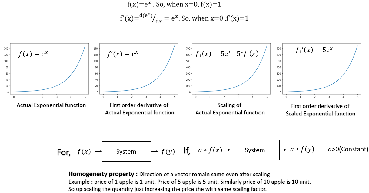
Even after scaling (multiplying by a constant), the rate change of the function remains the same as the original function. See, all the four curves above all look the same alike, right? Now let’s consider another exponential function like below.

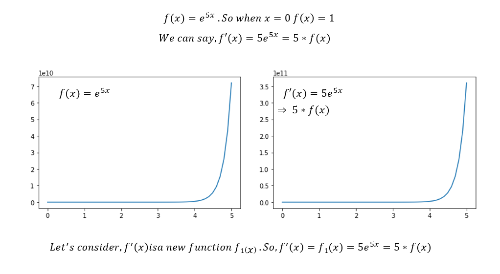
So what we get here is that by using derivative operates on our above exponential function, the result is the same original function multiplied by some constant number, which is 5 in this case. Now here, our f₁(x) is the eigenfunction of the derivative operator, and the constant number 5 is called the eigenvalue corresponding to the eigenfunction of the derivative operator. Now, how many eigenvalues are possible for our prementioned exponential function? Well, it’s infinite. So, we can say that our exponential function for the derivative operator has a continuous space of all possible eigenvalues known as spectrum. The conception of an eigenvalue and function is the most basic foundation of Fourier analysis or any linear transform. But let me give you a real-life example to understand the topic. Observe the below images with two birds.

How can you identify and separate if it’s an Owl or Eagle? Well, it will by its body, leg, face, etc. So, what are these components? These principal or characteristic features help us separate and identify an owl or Eagle. We can call these components dimensions. These principal or distinct components can be seen as eigenvectors, each having its elements. The leg will have colour, claw or body, type of feather, etc. Consider both images as a transformation matrix. The data (transformation matrix), when acted on the eigenvectors (principal components), will result in the eigenvectors multiplied by the scale factor (eigenvalue). And, accordingly, you can separate and identify the images.

Why do we need transformation? 

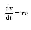
In the real world, how things are change over time often ends up as a Differential Equation, like in the case of Compound Interest. Money earns interest. The interest can be calculated at fixed times, such as yearly, monthly, weekly, etc., and added to the original amount. But when it is compounded continuously, the interest gets added in proportion to the current value of the loan (or investment). And as the loan grows, it earns more interest. Using t for time, r for the interest rate, and v for the current value of the loan:

Differential equations describe incremental changes dependent on other changes. If you have current state information, you can “playback” the system numerically in time, moment after moment(Integration).In the continuous domain, we are talking about infinite solutions, known as the Numerical technique. Where we are trying to approximate the value, it can be time-consuming. But for us, it is easy to comprehend a function with an exact solution like x2-4x+4=0 where x=2. It is known as the Analytical technique, which provides an immediate and clear solution as it usually requires less time to find a solution.

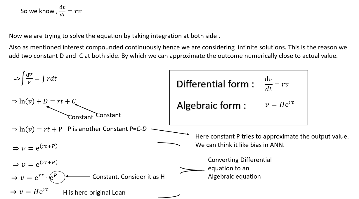
Also, when talking about “rate,” potential complexity increases by introducing more independent variables(Partial differential Equation). So, Differential equations can be hard to be solved analytically. So to have an analytical solution, we need to transform it into an algebraic equation.

Why Time-domain to Frequency domain?

When you hear a chord played from a musical instrument like Guitar, do you focus on its duration or what makes it sound the way it sounds? Time dictates when you hear something, but frequency dictates what you hear, which is much more central to the true nature of signals. Now let me give you another example. Let’s say you start recording your audio signal in a crowded, noisy area; the time instance starts from 0th second, and you stop after 30 sec. So, you have signal data for 30 seconds. Meaning, we have different voltage levels(Amplitude) for 30 seconds. Now, you want to segregate your voice from 13th second to 29th second. In this problem, how can you ensure that your extracted voice signal contains solely your voice but not the noise from outside? It can not be amplitude(one of the time-domain parameters) as you may speak with the same amplitude with external noise at that time. So what will be the differentiating parameter? The frequency. In the real world, the time domain only actually exists. The moment we are born, our experiences are developed we calibrate ourselves with the time domain. We are used to seeing events happen with a timestamp and ordered sequentially. An essential quality of the frequency domain is that it is not real.

Linear and Non-Linear System

Most of the systems we see in the real world are nonlinear means the input-output graph is not a straight line, and the graph of a nonlinear function is a curved line. The output change is not proportional to the input change in a nonlinear system. Nonlinear
systems are one of the biggest challenges and not easy to control because the nonlinear characteristic of the system abruptly changes due to some slight changes of valid parameters, including time, which leads to Chaos. The mathematical
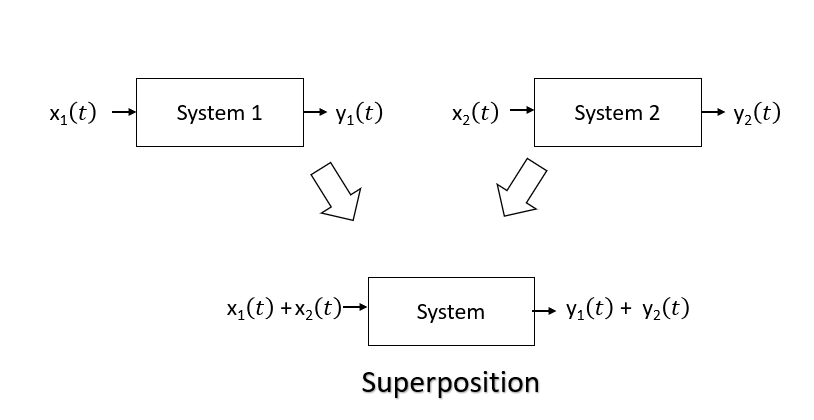
calculation is challenging for this type of system. It is the reason we try to convert any nonlinear equation to linear form. Linear system has two properties one I had said before Homogeneity, and another one is Superposition. The Superposition
is an additive function. You can have some intuition from the below diagram.

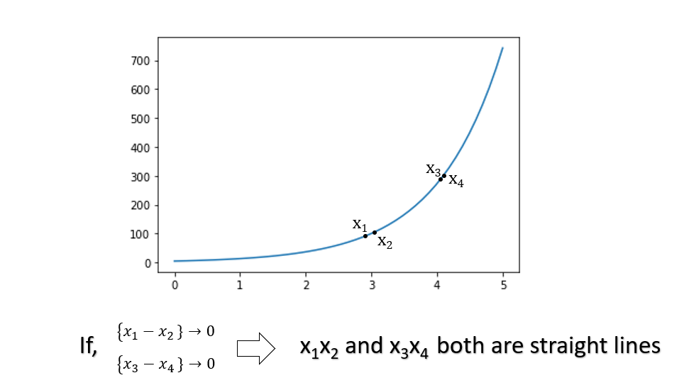
If we consider a nonlinear equation, it will have some curve format. But in a tiny region of point, the curve is almost linear. So, we can approximate a curve by considering it to be a straight line.

Folks already familiar with Fourier transformation, can you find some similarity in the linear system property x₁(t)+x₂(t)=y₁(t)+y₂(t).

Importance of Sinusoidal Signal

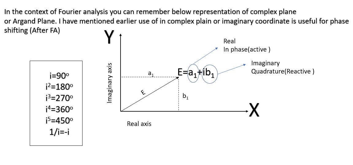
We have mentioned before exponential functions are proportional to their derivatives, meaning the y value of the function at a particular x value is equal to the slope of the curve at that same x value. Thus when dealing with exponential functions in calculus, e becomes a very natural number to use as a base. So, e^x has the property of being its derivative and eigenfunction. e^at is the eigenfunction of linear systems where the variable t is time. The constant a in the previous can be real, imaginary, or complex. From Euler’s formula, we know.

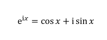
It speaks about imaginary exponent. The right side maps the angle x to the complex unit circle at angle x to the standard ray, the positive X-axis. The left side says e^ix is that same point on the unit circle. As per Euler’s Formula, angles are imaginary exponents, and angles are logarithms. When we multiply complex numbers, we add angles. This transformation of multiplication to addition is the primary property of exponents, of logarithms.

Since Euler’s relationship gives the below formulas,

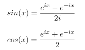
Here i is an imaginary number i² =-1

 Then since the two terms on the RHS fit the above eigenfunction statement regarding exponential function, then Sin(x) is an eigenfunction. We have spoken about Linear systems. Sinusoids are eigenfunctions of linear time-invariant systems. That means sinusoid yields sinusoid out with the same input frequency, gain-adjusted and phase-shifted. Also, when Sines and Cosines travel together in the form of e^ix=cos(x) + i[sin(x)], they become so-called “eigenfunctions” of the time translation operator. For this case, the frequency is constant. It is the main reason why Fourier analysis works.

Fourier Analysis 

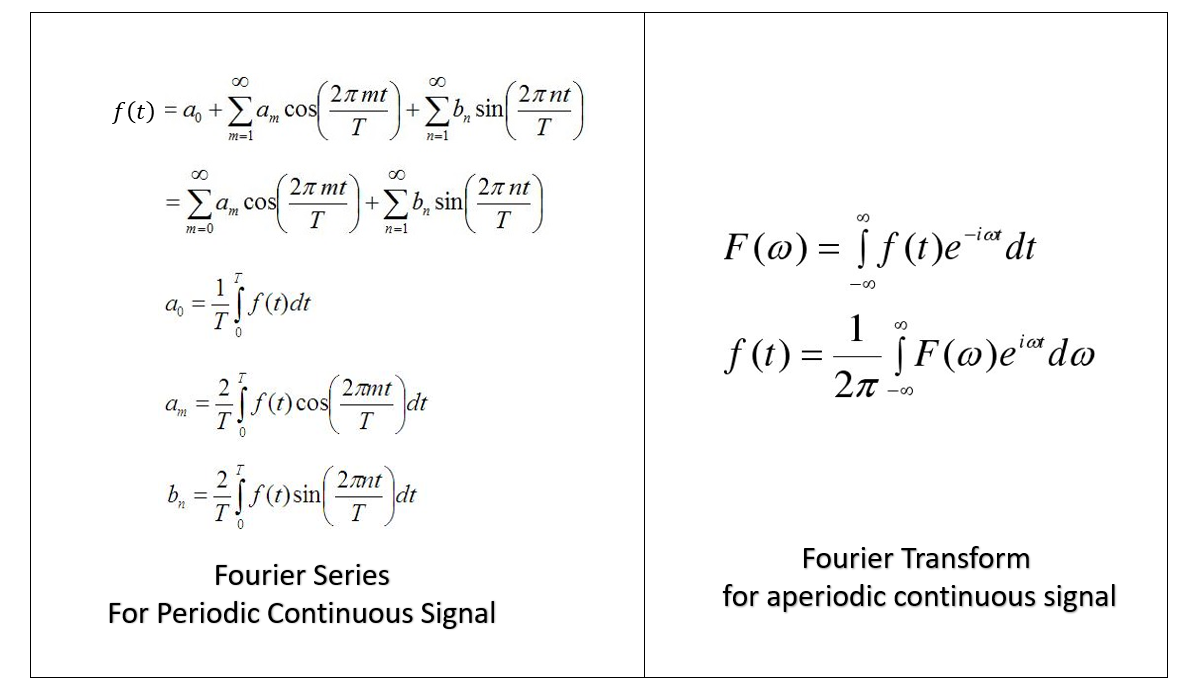
I think most of us are already aware that we convert the time domain to its frequency domain in the case of Fourier analysis. Previously I have described that why we need that. Now Fourier analysis can be done for periodic and nonperiodic signals. We use the Fourier series for periodic signals, and for the nonperiodic signal, we use Fourier transformation. While the Fourier series gives the discrete frequency domain of a periodic signal, The Fourier transformation gives the continuous frequency domain of a nonperiodic signal.

Fundamental Frequency

While studying Fourier analysis, one essential concept to understand is Fundamental Frequency. The applicability of the Fourier analysis is very vast; any time series data can be transformed by using this mathematical tool. To make you understand Fundamental Frequency, let me give you an example from the field of speech processing. While we are speaking, our vocal cords create an almost periodical vibration due to the opening and closing it. It is the reason the emitted speech sound is periodic. Even though it’s not sine in nature as long as it’s periodic, the sound we produce can be analyzed as a sine wave of the fundamental frequency plus harmonics of 2, 3, 4, etc. times the actual using the technique of Fourier series. So if you have a total of 300 Hz, the harmonics would be 600 Hz, 900 Hz, 1200 Hz, etc. So we can say The lowest frequency produced by any particular instrument is known as the fundamental frequency.

Prelude of Fourier Series

Before we begin, let me give you some intuition about some basic concepts. What do we mean when we say that signal period is 2π. It means the signal repeats its values on regular intervals, or “periods.” which is, in this case, is 2π. So, If Sin (π) = 0 and the period of the sine wave is 2π, then if you add 2π to the time domain, we will get (2π +π)=3π. So, sin(π), sin(3π) = 0 and so on. so we can say for basic function y=sin(x) the period is 2π. But in case x is multiplied by any number greater than 1, then the function will speed up, and the period will be smaller. Like y=sin(2x).In this case, the period is π. If x is multiplied by any number between 1 and 0, the period will be bigger than if x is multiplied by any number greater than 2π. To get the period for ​y​ = Sin (​nx​), you can use Period= 2π/|n|. The only thing that matters over here is the term associated with x.

What is the Fourier series?

Fourier Series is a method by which we approximate arbitrary periodic function (f(x)) as an infinite sum of sines and cosines of increasingly high frequency that provide an orthogonal basis for the space of solution functions. The sine and cosine functions are present as eigenfunctions of the heat equation.

Important conceptions before Fourier Series

When I first started reading about the Fourier series, one question that came into my mind was the basic function? To know this, we need to get acquainted with a few more mathematical terms, which I’ll try to explain in a simple format.

Vector, Vector Space, Basis, and Orthogonal Basis

Numbers 0–9 and their combinations are sufficient to represent Integers. Similarly, alphabets A-Z and their combinations are sufficient enough to represent writing in the English language. So, we can say that 0-9 are the basis of Integer Space or A-Z of English language Space. Well, I have just given you the intuition of Vector space with their basic objects. All these spaces have some of their rules, like English language space. Like Letters are combined to form words. Words are combined to form sentences. Sentences are combined to form paragraphs. Paragraphs are combined to form chapters/books/letters/blogs etc. So all the letters, words, sentences, paragraphs needed to be continuous, and they must follow some grammar and punctuation rules. Also, you have to write from left to right. Here A-Z can be considered as vectors.

In Mathematics, a vector space is a collection of mathematical objects called Vectors (not the typical vectors that we use in physics) that can be added together and multiplied by scalars. I had written just now, can you see something that I had described before while discussing the linear system?

For a 2D Vector space(X-Y plane), the standard vectors x(1,0), y(0,1) representing each of the axes are the basis. Using combination(addition) of x, y any vector in the 2D vector space can be conceived. Similar for a 3D Vector space(X-Y-Z cube), the standard vectors x(1,0,0), y(0,1,0), z(0,0,1) representing each of the axes are the basis. Using combination(addition) x,y,z any vector the 3D vector space can be conceived.

Now let us consider the 3D vector space axis X and Y. What is the inner similarity? Which is known as the inner product. By which we find the distance between them basis on an angle. Observe the below image.

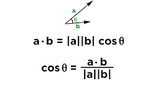
So, what you will multiply the corresponding basis value like for X(x1=1,y1=0,z1=0) and Y(x2=0,y2=1,z2=0) and Since x1.x2=1.0=0, we can say the angle between X and Y is 90 degrees ( We are omitting the calculation of denominator). Means X and Y are orthogonal. So, Here X and Y are orthogonal basis vectors. We can say that a basis of an inner product space is orthogonal if all of its vectors are pairwise orthogonal.

Vector Norms

Now, let’s consider we have defined a vector-like below in complex plain(Argand diagram). And see how we find the vector’s magnitude (3+4i ).

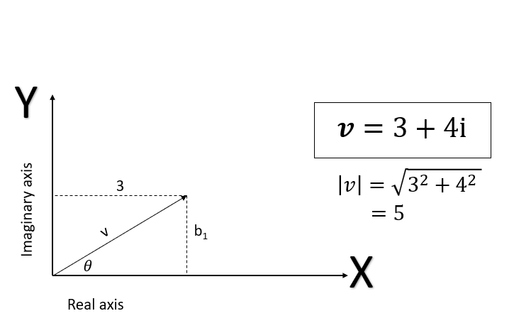
So, we are trying to find out the magnitude of the vector by using the Pythagorean theorem. We can extend this rule ( Pythagorean theorem)into higher dimensional vectors in the same way. So, this is a rule, or it is a Norm. So, We can say A norm is a map from a real value(R) or Complex Value(C) vector space V to Real Value(R). Now it has some axioms of Positive definite, Homogeneity, and Triangle inequality, which I will not describe here.

Hilbert Space and Fourier Series

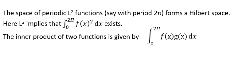
Now whatever I had discussed from vector space to vector norm, the reason for that is those were the prelude of Hilbert space which is the primary basis of Fourier series or Fourier Analysis. Let’s understand what exactly it is. We are familiar with 2D and 3D, consisting of the X-Y and X-Y-Z axis, respectively. We know that the shortest distance between two points will be the straight line connecting them. In 2D space, we use the Pythagorean theorem to calculate the distance, which is the hypotenuse. Here 2D and 3D space are Hilbert space. The remarkable thing about it is that Hilbert Spaces can have infinite dimensions. If we calculate the distance with finite spaces(2D), it won’t converge. Most distances will be indefinite or undefined. A single point represents a function in Hilbert space, whereas the space represents continuous functions. Every vector operation has to be evaluated with integrals because it’s a constant function space. The difference between Euclidean vector spaces is that you have to make the inner production an integral and apply the complex inner product formed via complex conjugation. Another function space would be the space of periodic functions, where you have sine and cosine as the basis. Hilbert space relates to the Fourier series. You don’t consider a single operation in isolation but instead consider the entire vector space of L² functions, which is, in fact, a Hilbert space. Here, L² denotes the set of complex-valued, square-integrable functions on the real line (i.e., functions f such that |f|² is integrable). More generally, L²(X) denotes the square-integrable functions on X.

Fourier Series Coefficients

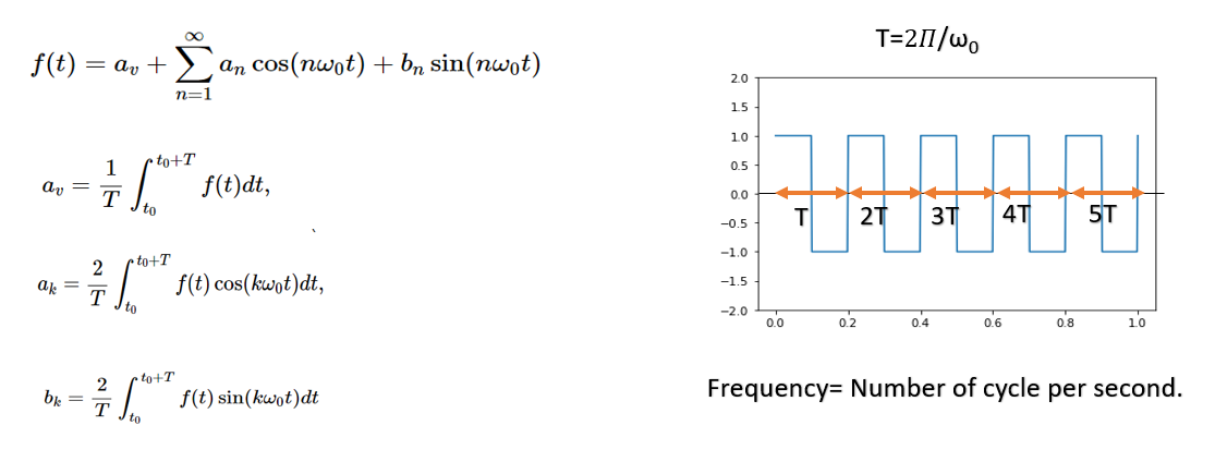
The Fourier Series function (f(x)) represented as a periodic function. Any periodic function with period L exhibits the same pattern after interval L along the X-axis. Consider X here as the time axis where the Numerical approximation of the Fourier Series function of a periodic function looks below where a_v, a_n, b_n are Fourier Coefficients. Also, The term ω₀ ((2Π/T)  represents the fundamental frequency of the periodic function f(t). The integral multiples of ω₀ like, 2ω₀, 3ω₀, 4ω₀ So on are known as the harmonic frequencies of f(t). nω₀ is the nth harmonic term of f(t).

Dirichlet’s conditions

For a periodic function f(t) to be a convergent Fourier series, the following conditions need to be met:

· f(t) be single-valued.

· f(t) has a finite number of discontinuities in the periodic interval.

· f(t) has a finite number of maxima and minima in the periodic interval.

· The integral of f(t) must exist with the lower and upper limits of the period.

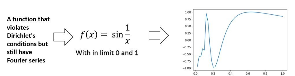
The above condition is known as the Dirichlet condition. If any function satisfies the Dirichlet condition, then every point of a function that we have given and the function we get by the linear combination of sine and cosine wave of different frequency is the same except at the point discontinuity. Also, Dirichlet Condition is unnecessary; some functions do not satisfy Dirichlet but still have the Fourier series. If the function satisfies the Dirichlet condition, it confirms that it has Fourier representation.

Code Part

# Python example - Fourier transform using numpy.fft method
import numpy as np
import matplotlib.pyplot as plt
# How many time points are needed i,e., Sampling Frequency
# The frequency at which a data set is sampled is determined by the number of sampling points per unit distance or unit time,
#and the sampling frequency is equal to the number of samples (or stations) divided by the record (or traverse) length.
#For example, if a wave-form is sampled 1000 times in one second the sampling frequency is 1 kHz (and the Nyquist frequency 500 Hz);
#if a traverse is 500m long with 50 stations, the sampling frequency is one per 10 m.
samplingFrequency  = 50;
# At what intervals time points are sampled
samplingInterval= 1 / samplingFrequency;
# Begin time period of the signals
beginTime = 0;
# End time period of the signals
endTime  = 8; 
# Frequency of the signals
signal1Frequency     = 3;
signal2Frequency     = 6;
# Time points
time= np.arange(beginTime, endTime, samplingInterval);
# Create two sine waves
amplitude1 = np.sin(2*np.pi*signal1Frequency*time)
amplitude2 = np.sin(2*np.pi*signal2Frequency*time)
# Create subplot
figure, axis = plotter.subplots(4, 1)
plt.subplots_adjust(hspace=1)
# Time domain representation for sine wave 1
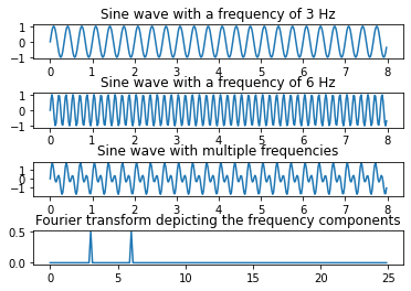
axis[0].set_title('Sine wave with a frequency of 3 Hz')
axis[0].plot(time, amplitude1)
# Time domain representation for sine wave 2
axis[1].set_title('Sine wave with a frequency of 6 Hz')
axis[1].plot(time, amplitude2)
# Add the sine waves
amplitude = amplitude1 + amplitude2
# Time domain representation of the resultant sine wave
axis[2].set_title('Sine wave with multiple frequencies')
axis[2].plot(time, amplitude)
# Frequency domain representation
fourierTransform = np.fft.fft(amplitude)/len(amplitude)           # Normalize amplitude
fourierTransform = fourierTransform[range(int(len(amplitude)/2))] # Exclude sampling frequency
tpCount     = len(amplitude)
values      = np.arange(int(tpCount/2))
timePeriod  = tpCount/samplingFrequency
frequencies = values/timePeriod
# Frequency domain representation
axis[3].set_title('Fourier transform depicting the frequency components')
axis[3].plot(frequencies, abs(fourierTransform))
plt.show()

 

Digital frequency and Analog frequency 

In the case of Continuous Signal signal, it can take continuous values in both amplitude and time. For example, if a certain point in the signal has a value of 3.8, it will take all the other values closer to the prementioned value of 3.79,3.799,3.7999,3.79999. Till infinity. It means taking all the real values both in the amplitude size and time side. For example, at 3.2 seconds, it is taking the value of 3.8, then similarly in time also it will have continuous values such as 3.19,3.199,3.1999 up to infinity. Whereas in Discrete Signal, it will have constant values in Amplitude domain, but Discrete, i.e., countable values in Time domain. So the time domain will take integer values like -3,-2,-1,0,1,2,3 till n where n is the finite time. A Discrete signal is usually obtained by sampling the continuous signal and is the first step to convert any Continuous Signal to a Digital Signal. A band-limited signal can be reconstructed precisely if sampled at a rate at least twice the maximum frequency component in it(Nyquist sampling theorem). Oversampling occurs when we sample at a frequency much higher than the critical frequency (twice the highest frequency component). Under-sampling or aliasing occurs when the sampling frequency is less than the required frequency. Let’s clear the intuitive difference between digital frequency and analogue frequency. Digital frequencies are unit cycles/sample, while analogue frequencies have unit cycles/second. As per the Nyquist sampling theorem, when you digitize an analogue signal of bandwidth W, the sampling frequency must be at least double (2W) (or the distance between samples is 1/2W) to guarantee reconstruction. For example, for speech spectrum is bounded at 20 kHz, a typical sampling rate is 44.1 kHz.

You can refer to the below link for a better understanding.

https://www.kaggle.com/faressayah/signal-processing-with-python

Laplace and Z Transformation

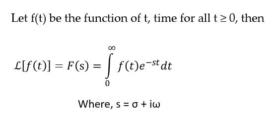
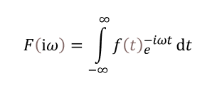
Some functions won’t be having Fourier Transformation. Like, if a process grows exponentially with time. Then it has no Fourier transformation. How can you solve this problem? Multiply the original function by a decaying exponential that decays faster than the primary growth function, and now you can have a function that has a Fourier Transform! The Fourier Transformation of that new function known as Laplace Transformation is evaluated on a complex plane parallel to the imaginary axis.

Just remember one thing [ ] denotes discrete signal and ( ) represents the continuous signal.

Now, the Laplace transform is very similar to the Fourier transform. While the Fourier transform of a function is a complex function of a real variable (frequency), the Laplace transform of a function is a complex function of a complex variable. Laplace transforms are usually restricted to functions of t with t > 0.

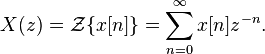
I will not give you a detailed explanation of the Z transform. Just remember Z transform is used to convert the discrete time-domain signal into a discrete frequency domain signal.

The continuous-time Fourier transform is a particular case of the Laplace transform, and the Discrete-Time Fourier transform is a specific case of the Z-transform. It means that Laplace and Z Transformation can manage systems and equations that Fourier transform cannot.

In Z transformation, there is a conception of the Region of convergence(ROC). Which is defined as the set of points in the complex plane for which the Z-transform summation converges. So, ROC={z:∥(∑∞n=−∞x[n]z−n)∥<∞}. So for a signal, if the Region of convergence encloses the value ∥z∥=1, then the Laplace and Fourier transform for that signal will exist. The Z-transform will live even if the Fourier and Laplace transform exists. When taking  Z-transform of signal and it’s limited to the circle ∥z∥=1, it is called a Laplace transform, and if it’s limited to the point, z=e^−iω.

Discrete-Time Fourier Transform (DTFT) and Discrete Fourier Transform(DFT)

A function in the time domain is known as a signal, and a function in the frequency domain is known as a spectrum. DTFT is a theoretical conception where a Discrete, aperiodic time-domain signal is transformed into a continuous, periodic frequency-domain signal. You can consider DTFT as Time-discrete, Fourier transforms, and it is an infinite length nonperiodic sequence to complex-valued 2π periodic frequency components. We can define DTFT as below.

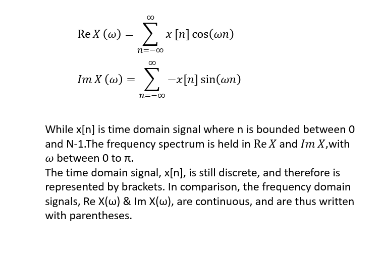
The frequency variable is continuous, but since the signal itself is defined at discrete instants, the resulting Fourier transform is also represented at the time. The number of time points will still be infinite, and it is just that you would have a finite number of points between any two-time point.

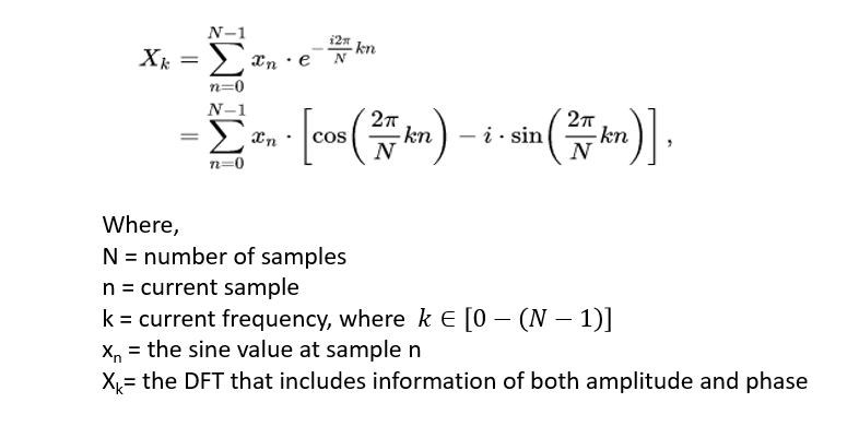
The output of DTFT is continuous, Mathematically even though it’s correct, but in real life, it is not practical. So we have to convert this constant signal into discrete form. DFT maps one infinite and periodic sequence, x[n] with period N in the “time” domain, to another unlimited and periodic sequence, X[k], again with period N, in the “frequency” domain.

We will discuss more DFT here. But before we proceed, let us understand another few more essential conceptions.

Impulse Response

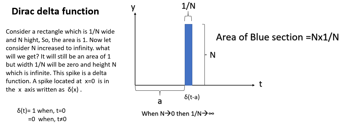
The impulse response is a short-duration time-domain signal. For continuous-time systems, this is the Dirac delta function δ(t), Incase of discrete-time systems, the Kronecker delta function δ[n] is mainly used. A system’s impulse response (often annotated as h(t) for continuous-time systems or h[n] for discrete-time systems) is defined as the output signal that results when an impulse is applied to the system input. You can guess why this function is vital if you see the illustration below.

It allows us to predict what the system’s output will look like in the time domain. If we can decompose the system’s input signal into a sum of many components, then the output is equal to the sum of the system outputs for each of those components. So, if we can decompose our input signal into a sum of scaled and time-shifted impulses, the output would be equal to the sum of copies of the impulse response, scaled and time-shifted in the same way, which is a property of the LTI system.

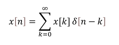
For discrete-time systems, this is possible because you can write any signal x[n] as a sum of scaled and time-shifted Kronecker delta functions.

Each term in the sum is an impulse scaled by the value of x[n] at that time instant. Each scaled and time-delayed impulse that we put in yields a scaled and time-delayed copy of the impulse response at the output. That is:

Where h[n] is the system’s impulse response, the above equation is the convolution theorem for discrete-time LTI systems. For any signal x[n] input to an LTI system, the system’s output y[n] is equal to the discrete convolution of the input signal and the system’s impulse response. This can be done for Continuous.

So, I am saying all these because a system’s frequency response is the impulse response transformed to the frequency domain. If you have an impulse response, you can use the FFT to find the frequency response, and you can use the inverse FFT to go from frequency response to an impulse response.

Convolution and Correlation

Let us look at a discrete-time system how delta function looks like; as per my previous description, you can consider any signal x[n] as a sum of a time-shifted and scaled delta function(can be called as Kronecker delta functions). So, it will be like below.

Or we can write like below,

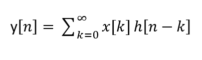
Here h[n] is the system’s impulse response. Both of the above equation projects the convolution for discrete-time LTI systems. Meaning, for any signal, if x[n] is the input to an LTI system, the output y[n] will be equal to the discrete convolution of the input signal and the system’s impulse response.

Convolution is the degree of overlapping of the areas of the two signals that are being convolved. Whereas Correlation helps to tell the degree of similarity between two objects or signals. Lets have an intuition of correlation first consider following coordinate C1=(x1,y1),C2=(2×1,y1),C3=(x2,y2),C4=(-3×2,y2). We can see between C1 and C2, and there is a relation if x1 for C1 increases, x1 in C2 will increase like if C1=(2,3) then C2=(4,3). So, there is a relation between a positive direction; C1 and C3 do not hold any relation. C3 and C4 are related as x2 in C3 increases, the x2 in C4 always decreases three times. We can say C1 and C2 are positively correlated. C1 and C3 are not correlated. At the same time, C3 and C4 are negatively correlated.

Now consider that C1, C2, C3, and C4 are part of the same signal(like a square pulse wave), this type of Correlation is auto-correlation. And if C1 and C3, let’s say part of signal A and C2 and C4 are part of signal B, then we call it cross Correlation.

Now convolution is the way you hear sound in a given environment (room, open space, etc.) is a convolution of an audio signal with the impulse response of that environment. In this case, the impulse response represents the characteristics of the environment like audio reflections, delay, and speed of audio which varies with environmental factors. Convolution arises when we analyze the effect of multiplying two signals in the frequency domain. If we multiply two signals in time, the Fourier representation for the product is the convolution of the Fourier representations of the individual signals. Remember, a convolution kernel is a correlation kernel rotated 180 degrees. I leave it here so that you can do some research on it.

Discrete Fourier Transformation (DFT)

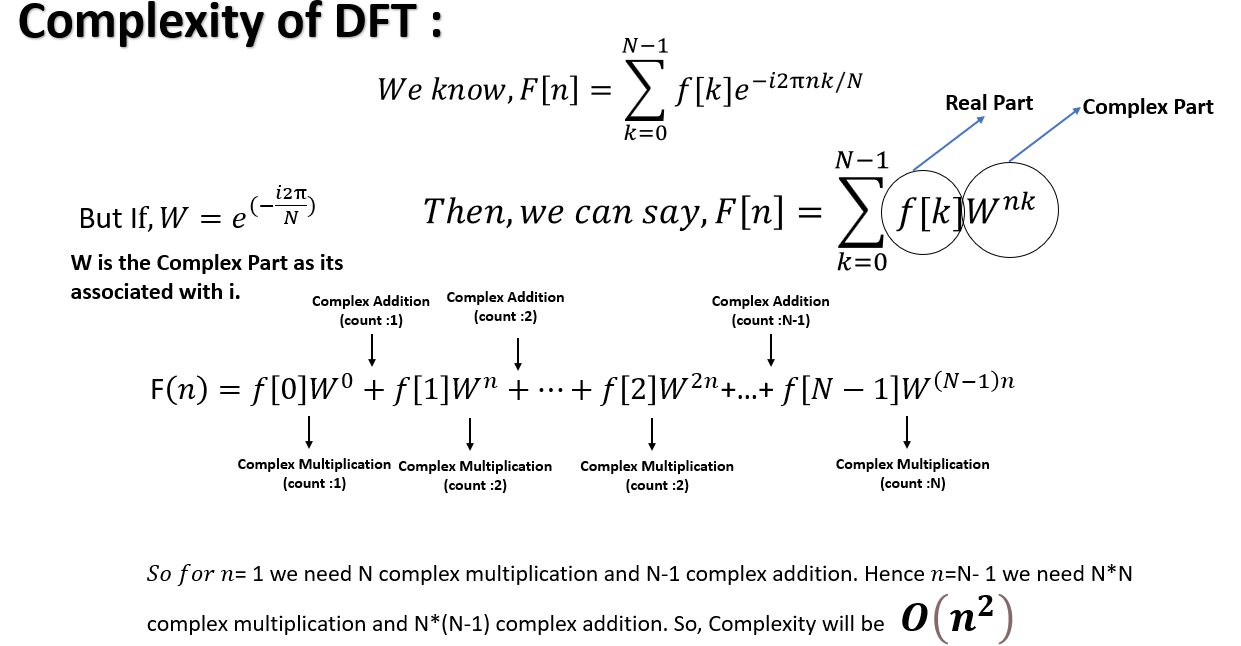
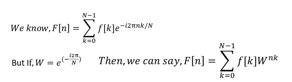
DFT or Discrete Fourier Transformation is a continuous Fourier transform for a signal where the main signal f(t) has a finite sequence of data in the time domain. DFT is a Fourier series that works on a discrete frequency axis, s Since it uses only a finite set of frequencies, it is a Discrete Fourier Series. Here, F(0) is the D.C. component. F(1) is the fundamental frequency(Sampling frequency) component. F(2) is the second harmonic (twice the sampling frequency) and so on. DFT works by measuring the Correlation with an integer multiple of frequencies. If the frequency exists, the Correlation is 1 else zero. Different integer multiple frequencies are windowed on a discrete sequence. The perfect match (Correlation) is the frequency present in the signal. Let’s consider N instances are separated by sample time T. Here f(t) is continuous signal and also lets assume N samples are represented as f[0],f[1],f[2],…f[k]….f[N-1]. So, the Fourier transform of the original signal f(t) will be.

We consider each sample f[k] impulse of the signal having area f[k]. Then we can write,

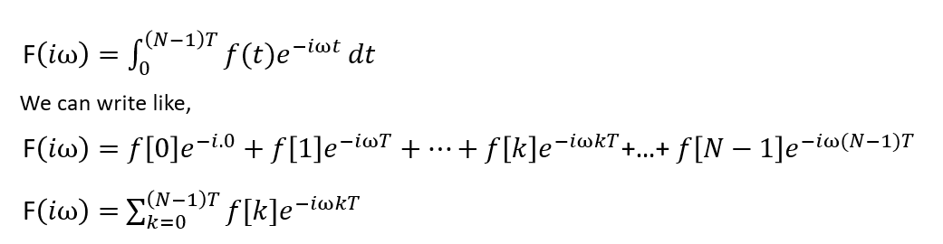
We know that we can evaluate continuous Fourier transform over a finite interval ( the fundamental period T₀) rather than from – ∞ to +∞ if the signal is periodic. Similarly, since there are only a limited number of input data points, the DFT treats the data as if it were periodic means from f(N) to f(2N-1) is the same as f(0) to f(N-1)

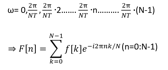
Since the operation treats the data as if it were periodic, we evaluate the DFT equation for the fundamental frequency (one cycle per sequence, 1/NT Hz,2π/N.T. rad/sec and its harmonics at ω=0.

So,

Vandermonde matrix representation of DFT

First, let me give you an intuition of the Vandermonde matrix. Consider we have 04 coordinates like (1,7),(2,3),(-2,4),(0,9). Now you have to find a polynomial f(x) that passes through all of these points.

so, we can write f(1)=7,f(2)=3,f(-2)=4,f(0)=9.

Since we have 04 points to consider a polynomial we can consider a cubic polynomial Like f(x)=ax³+bx²+cx+d( for 03 given points you can consider square polynomial so for N points you can consider a polynomial of N-1)

Lets consider our cubic polynomial.

f(1)=a(1)³+b(1)²+c(1)+d=7

f(2)=a(2)³+b(2)²+c(2)+d=3

f(-2)=a(-2)³+b(-2)²+c(-2)+d=4

f(0)=a(0)³+b(0)²+c(0)+d=9

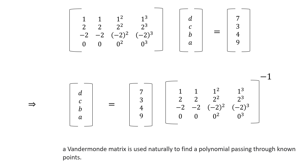
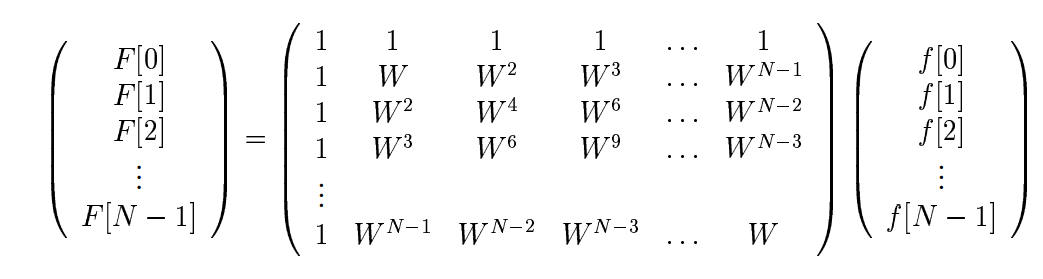
Now we know F[n]is the Discrete Fourier Transform of the sequence f[k]. We may write this equation in matrix form (Vandermonde matrix representation) as:

Code Part

import matplotlib.pyplot as plt
import numpy as np
# sampling rate
sr = 100
# sampling interval
ts = 1.0/sr
t = np.arange(0,1,ts)
freq = 1.
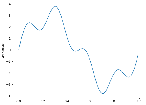
x = 3*np.sin(2*np.pi*freq*t)
freq = 4
x += np.sin(2*np.pi*freq*t)
plt.figure(figsize = (8, 6))
plt.plot(t, x)
plt.ylabel('Amplitude')
plt.show()
def DFT(x):
    """
    Function to calculate the 
    discrete Fourier Transform 
    of a 1D real-valued signal x
    """
    N = len(x)
    n = np.arange(N)
    k = n.reshape((N, 1))
    e = np.exp(-2j * np.pi * k * n / N)
    X = np.dot(e, x)
    return X
X = DFT(x)
# calculate the frequency
N = len(X)
n = np.arange(N)
T = N/sr
freq = n/T 
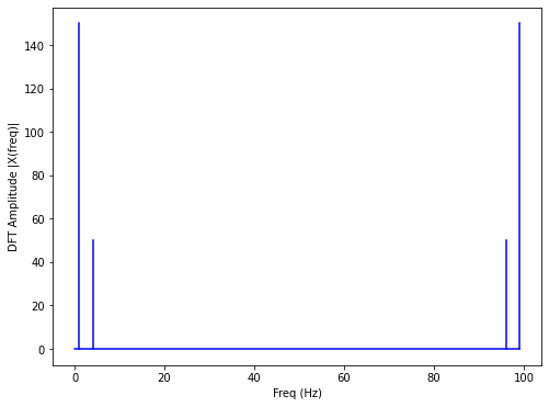
plt.figure(figsize = (8, 6))
plt.stem(freq, abs(X), 'b', 
         markerfmt=" ", basefmt="-b")
plt.xlabel('Freq (Hz)')
plt.ylabel('DFT Amplitude |X(freq)|')
plt.show()

Twiddle Factor and Time Complexity of DFT

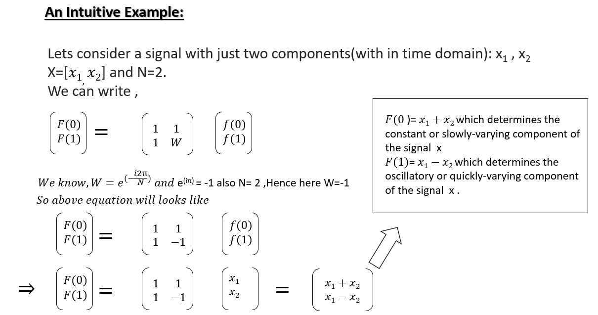
W is called a twiddle factor means rotating vector quantity. Also, we can say a twiddle factor is a complex number whose magnitude is one. As such, multiplying a complex number whose magnitude is M by a twiddle factor produces a new complex number whose magnitude is also M. I think the below image will give you an intuition of it.

Fast Fourier Transform (FFT)

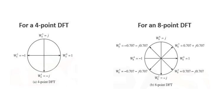
Fast Fourier Transform (FFT) algorithms rely on the standard DFT involves many redundant calculations.

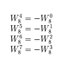
The integer product nk repeats for different combinations of k and n secondly. Also, we can say W^nk is a periodic function. The integer product nk repeats for various blends of k and n. Secondly. Also, we can say it is a periodic function with only N distinct values. For better clarification, observe the Twiddle Factor image. For Twiddle factor for 8 point DFT, we can say,

FFT Algorithm 

From above, we can say there is a relation between the odd and even power of W. We can split the summation over N samples into 2 summations, each with N/2 samples, one for k even and the other for k odd. So replace m=k/2 for k is even and m=(k-1)/2 for k is odd. Then

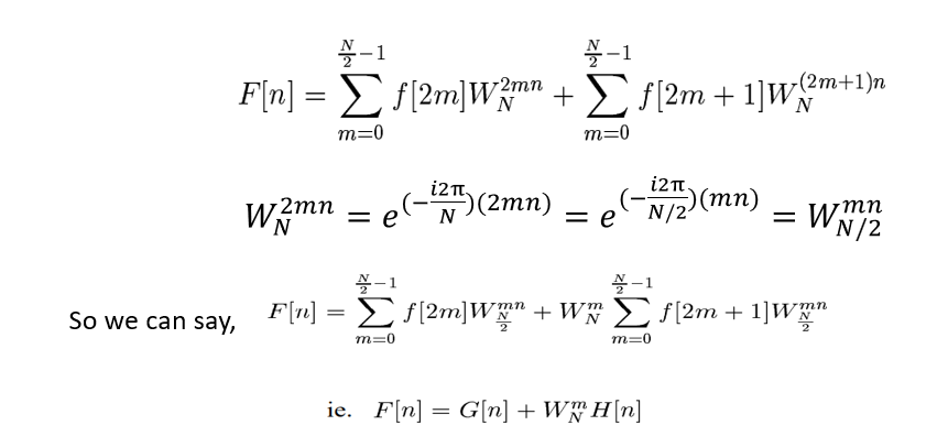
So we can say N-points DFT F(n) can be obtained from two N/2 point transformations. Here G[n] for even input data and H[n] for odd input data. Here G[n] and H[n] are periodic in n with period n/2.

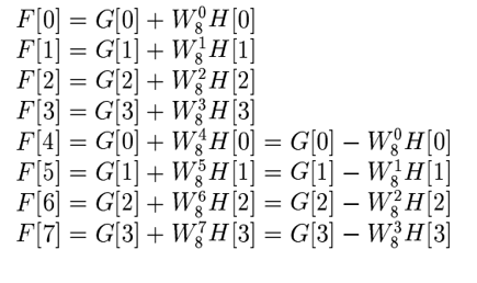
If N=8, we can say

Even input = f[0],f[2],f[4],f[6],f[8]

Odd input = f[1],f[3],f[5],f[7]

We can write like below :

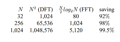
We have used the approach to divide and conquer the same as a binary search algorithm in the data structure. At each stage of the FFT, we need N/2 complex multiplication to combine the result of the previous stage. And We can see there is a log₂ N stage. So, the number of multiplication required is N/2log₂N.

For the coding part of FFT, you can refer to blog link.

Conclusion

Well, this content is kind of an epic if you possibly managed to read the entire guide on Fourier Analysis. While reading it, you may feel that you are watching the movie “Inception.” But If you can connect the dots hope this article will help you. Also, on the last note, I like to mention. Why do we need transformation at all? I was reading an article one guy had simplified it marvellously. I will give an example for the same before ending it. Lets, Consider a=2873658 and b=8273645, and you have asked to do multiplication(think of it as convolution) of the numbers. How easily can you do that? If you take a logarithm, then log(ab) will become log a+ log b. is it not simplifying the multiplication? You can consider taking long as equivalent to Fourier Transform, Z transform, or Laplace transform.

Hope this guide on Fourier Analysis was enriching. If you like to read more articles, then head on to our blog.

References

Image sources

The media shown in this article is not owned by Analytics Vidhya and are used at the Author’s discretion. 

Subhasis Sanyal 10 Jan 2022