This article was published as a part of the Data Science Blogathon.
Introduction
Emotions are expressed through words, gestures, expressions, and with the ease of accessibility of social media today, emotions can now, also be expressed through tweets and Instagram/ WhatsApp stories.
Through this article, we would try to analyze the underlying emotions of tweets posted by people, you can find the dataset here.
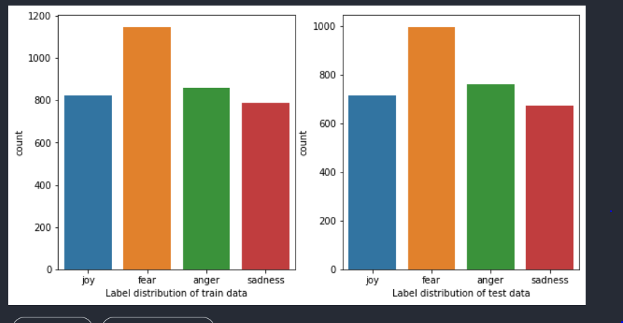
We first check if the distribution of classes in both the train and test datasets is the same or different. Sometimes when the distribution of classes is not the same in both train and test sets, it might affect the model’s performance on test/unseen data, it is a good practice to check the distribution before going ahead with building models. Also, knowing the distribution of classes in your data can help you in choosing a good metric for your problem, take the case when you have imbalanced classes in your dataset, accuracy might not be the metric you would want to use, because accuracy can give you misleading results. For example, when you have 90 samples from the positive class and 10 samples from the negative class, if your model is dumb that is, it classifies all samples as positive, you would have an accuracy of 90%, which gives a false impression of the model’s performance.
As can be seen from the below figure distribution of labels in both train and test datasets is similar and the data is fairly balanced.
Using Word Counts as a Feature
Let us see if the word count of the tweets has a relationship with the underlying emotion being depicted. In general, we would expect an angry tweet to be lengthier than a happy tweet, through the below code we try to identify if our intuition does hold.
def word_count(df):
    word_count = []
    for i in df['text']:
        word = i.split()
        word_count.append(len(word))
    return word_count
train['word_count'] = word_count(train)
test['word_count'] = word_count(test)
The above function splits the sentences into words and counts the number of words in the train and test datasets.
train_joy = train[train.label == 'joy']train_anger = train[train.label == 'anger']train_fear = train[train.label == 'fear']train_sadness = train[train.label == 'sadness']test_joy = test[test.label == 'joy']test_anger = test[test.label == 'anger']test_fear = test[test.label == 'fear']test_sadness = test[test.label == 'sadness']
The above code splits the train and test datasets based on their classes.
plt.figure(figsize=(20,5))
plt.subplot(1,4,1)
plt.plot(train_joy.word_count)
plt.xlabel("Word distribution of train data for class joy")
plt.subplot(1,4,2)
plt.plot(train_anger.word_count)
plt.xlabel("Word distribution of train data for class anger")
plt.subplot(1,4,3)
plt.plot(train_fear.word_count)
plt.xlabel("Word distribution of train data for class fear")
plt.subplot(1,4,4)
plt.plot(train_sadness.word_count)
plt.xlabel("Word distribution of train data for class sadness")
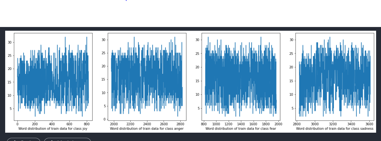
As is visible from the above graph range of words from tweets depicting joy are 0–800, tweets depicting fear are 800–2000, tweets depicting anger are 2000–2800 and sadness are 2800–3600.
A similar distinction of range can be seen in the test dataset as well. Find the below visualization.
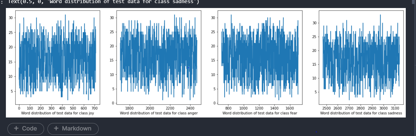
Since we have a different range of words for different emotions depicted by the tweet, we could try to use this word count feature by itself and train a simple Decision Tree classifier and measure the performance to validate if the feature is genuinely useful.
from sklearn import preprocessing
le = preprocessing.LabelEncoder()
y_train = le.fit_transform(train.label)
y_test = le.transform(test.label)
X = train['word_count'].values.reshape(-1,1)
X_test = test['word_count'].values.reshape(-1,1)
from sklearn.tree import DecisionTreeClassifier
clf = DecisionTreeClassifier(random_state = 5,max_depth=4,splitter='best')
clf.fit(X,y_train)
y_preds = clf.predict(X_test)
from sklearn.metrics import accuracy_score
acc_score = accuracy_score(y_test,y_preds)
print(acc_score)
We have used LabelEncoder to convert our target variable which is a categorical feature to a numeric feature, post that we have trained the DecisionTree classifier with a depth of 4, we get an accuracy of 30% which is not very good, so let’s try another model.
from sklearn.linear_model import LogisticRegression
lr = LogisticRegression(C=0.3)
lr.fit(X,y_train)
y_preds = lr.predict(X_test)
acc_lr_score = accuracy_score(y_test,y_preds)
print(acc_lr_score)
On training the logistic regression we get an accuracy of 31.66%, a slight improvement but not a great one.
As we could not get a good accuracy using word count, let us now use the text feature but before that, we would need to convert the text to numeric vectors. There are various ways to achieve the task, we would be following the below approaches as part of this case study.
1) Using CountVectorizer/ Bag of words model to convert the text to vectors.
2) Using TF IDF vectorizer to convert the text to vectors.
3) Using pre-trained embeddings to convert the text to vectors.
Using Count Vectorizer Model for Featurization of Text
Introduction to the BOW Model
Bag of words is a simple technique to convert text to vectors. In this technique, the term frequency of a word is replaced in place of the word. For example, if the original sentences are
1) Mary had a little lamb whose sheep was white as snow
2) Johhny Johhny, yes pappa!
as Mary is repeated only once in the entire corpus its term frequency is 1 and Johhny’s term frequency is 2.
Accordingly, the sentences would become (removing the punctuations) and considering the corpus is Mary had a little lamb whose sheep was white as snow Johhny yes pappa
1) [1,1,1,1,1,1,1,1,1,1,1,0,0,0]
2) [1,1,1,1,1,1,1,1,1,1,1,2,1,1]
The disadvantage of the BOW model is it does not consider the sequence of words, and as language does involve sequence and context, sometimes the BOW model might not be a good fit for the best-case scenario.
Let us see the code in action.
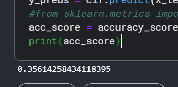
from sklearn.feature_extraction.text
import CountVectorizervect = CountVectorizer()
X_vec = vect.fit_transform(train['text'])
X_test_vec = vect.transform(test['text'])
clf.fit(X_vec,y_train)y_preds = clf.predict(X_test_vec)
#from sklearn.metrics import accuracy_scoreacc_score = accuracy_score(y_test,y_preds)
print(acc_score)
Output:

The above code uses the Count vectorizer which is an implementation of the BOW model by sklearn library to vectorize the text feature and then pass it to a decision tree classifier, as is visible from the above screenshot we get an accuracy score of 35.61%.
Next, we try the Random Forest Classifier model which is a bagging ensemble model technique to see if it improves accuracy. And voila! we get an accuracy of 81.1%.
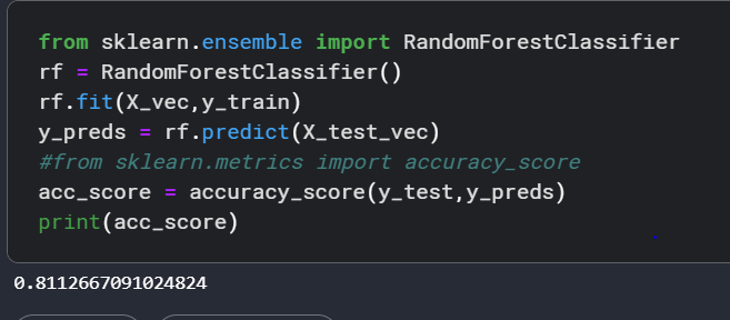
Random Forest Classifier uses low bias, high variance models(for example decision trees) as base models and then aggregates their output. Aggregation in classification can be done through techniques such as maximum voting in a classification scenario and taking averages in a regression scenario. You can read more about Random Forests here.
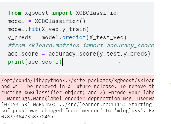
We next use the XGB classifier, the model belongs to the boosting ensemble model family. In boosting the main idea is to use high bias and low variance base models such as stumps which are low depth decision trees and feed the error of one model into another. In the end, what we get is a sequence of models trying to minimize the training error, you can read more about it here.
!pip install xgboost
from xgboost import XGBClassifier
model = XGBClassifier()
model.fit(X_vec,y_train)
y_preds = model.predict(X_test_vec)
#from sklearn.metrics import accuracy_score
acc_score = accuracy_score(y_test,y_preds)
print(acc_score)
We get an accuracy of 83% with the XGBoost model.
Using TF IDF Vectorizer for Featurization of Text
TF IDF vectorizer involves the multiplication of two values the term frequency and the inverse document frequency. The term frequency is simply as we discussed before the number of times a term occurs in a document. Inverse document frequency is calculated as log(number of documents in the corpus/ the number of documents that contain the term).
To break IDF of inverse document frequency down consider what would be document frequency of a term, simply the number of documents where the term occurs divided by the total number of documents in the corpus, and its inverse would be 1/document frequency, and when we take a log of it, that’s how we get the IDF formula, consider two terms ‘’problem’’ and ‘’misogyny’’.
In a corpus of 50000 documents if the term ‘’problem’’ occurs 500 times then log(50000/50000) would be log(1) which would be 0 and if misogyny occurs 10 times then 50000/10 would be log(5000) which would be 3.69.
Their TF IDF scores would become 500 * 0 for ‘’problem’’ which would be 0 and for ‘’misogyny’’ it would be 10 into 3.69 which would be 36.9.
The basic idea behind IDF is it rewards the rarity of words, if a word is present in all documents of a corpus it probably would not provide a lot of value as a feature than a word that is present only in some documents.
Let’s see if using TF IDF vectorizer, we can improve the accuracy of our emotion classifier 🙂
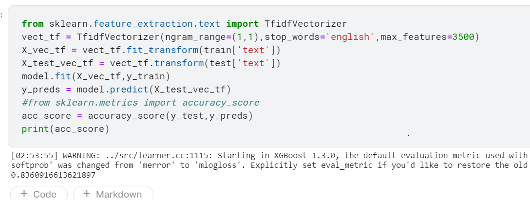
We first use the XGB Classifier we discussed earlier and get an accuracy of 83%, not a major improvement over what we had while using the count vectorizer.
from sklearn.feature_extraction.text import TfidfVectorizer
vect_tf = TfidfVectorizer(ngram_range=(1,1),stop_words='english',max_features=3500)
X_vec_tf = vect_tf.fit_transform(train['text'])
X_test_vec_tf = vect_tf.transform(test['text'])
model.fit(X_vec_tf,y_train)
y_preds = model.predict(X_test_vec_tf)
#from sklearn.metrics import accuracy_score
acc_score = accuracy_score(y_test,y_preds)
print(acc_score)
We use sklearn’s implementation of the TF IDF vectorizer, below are the explanations of parameters we have used.
1) ngram_range specifies the n-grams you would want to consider.
Consider the sentence: “I want to learn NLP.”
Unigram for this sentence would be I, want, to, learn, NLP
Bigrams for the same sentence would be I want, want to, to learn, learn NLP
SImply, we can say that n-grams are a collection of n sized chunks of words, with n-grams we can bring in some context of previous and next words which was completely absent in the BOW model.
2) stop words: Words like ‘an’, ‘at’, ‘the’ which are present very frequently in a set of documents but does not provide a lot of meaning to the interpretation of the sentence are called skew words, using this parameter lets our vectorizer know that we are to ignore all stopwords.
3) max features: These signify the top most important features that are to be included, since we have mentioned 3500, the best 3500 features would be considered by the vectorizer.
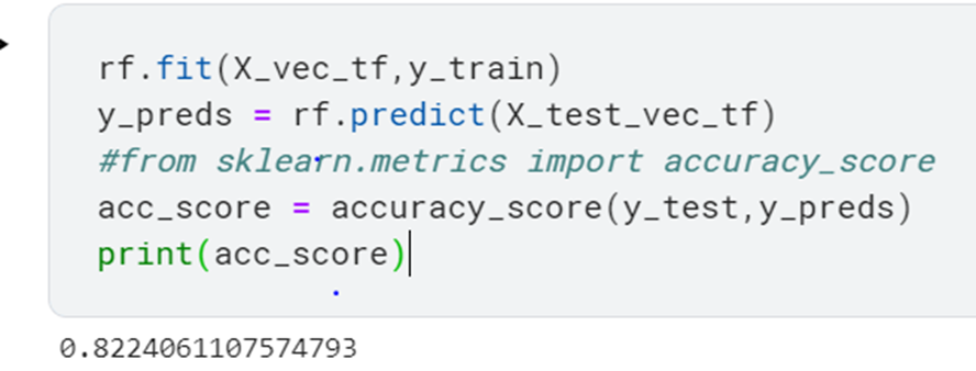
Next, let us try using the Random Forest model for the classification task.
rf.fit(X_vec_tf,y_train)
y_preds = rf.predict(X_test_vec_tf)
#from sklearn.metrics import accuracy_score
acc_score = accuracy_score(y_test,y_preds)
print(acc_score)
We get an accuracy of 82.24%
Using Pre-Trained Embeddings for Featurization of Text
Pre-trained embeddings function as a lookup for words to find their respective vectors, these embeddings are generated based on some underlying similarity.
For example, if you consider GLOVE embeddings, the word king and queen would share a similar relationship to man and woman in the vector space.
Using Universal Sentence Encoders(USE), we can encode the entire sentences to vectors just as simply as we encode words to vectors using GLOVE.
Let us see the code:-
import tensorflow_hub as hub
import lightgbm as lgb
def embed_document(data):
    model = hub.load("https://tfhub.dev/google/universal-sentence-encoder/4")
    embeddings = np.array([np.array(model([i])) for i in data])
return pd.DataFrame(np.vstack(embeddings))    # vectorize the data
X_train_vec = embed_document(X_train)
X_test_vec = embed_document(X_test)    # USE doesn't have feature names
model = XGBClassifier(n_estimators=1000,learning_rate=0.001,max_depth=5,n_jobs=8)
#print(X_train_vec.shape,y_train.shape)
model.fit(X_train_vec, y_train)
model.score(X_test_vec, y_test)
ypred = model.predict(X_test_vec)
print('XGBoost scores')
#score = roc_auc_score(ypred,y_test)
#print(score)
accuracy = accuracy_score(y_test, ypred)
print(accuracy)
print("-------------------------------------------------------------------")
We are loading the universal-sentence-encoder from the TensorFlow hub, note that we are not explicitly training the model as it is already pre-trained on a corpus we are just using it to create embeddings for our text in the train and test datasets.
We get an accuracy of 60 % which is lower than what we received for the count vectorizer model.
Conclusion
Though using pre-trained embeddings has its advantages such as lower training time, no requirement of finding a large number of documents to train the model from scratch, however, it does have some disadvantages some of them are out of vocabulary words or sentences, in the case your data has some words/sentences not seen originally by the model while it’s training, the model would not be able to generate appropriate embeddings for it, also if the context of documents on which your model is trained is different from your specific use case, such as if the pre-trained model has been trained on news dataset it would most probably perform poorly on another unrelated use case.
These might be the reasons why using a pre-trained embedding for our particular use case is not giving us a good result.
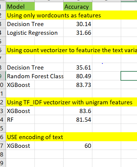
Considering the same, the best results we receive on our task are with XGBoost using count vectorizer, below is a table representing the results we received by using different techniques.
Read more blogs on NLP on our website.
A tiny bit about me:-
I am website, currently working as an analyst. By writing these articles I try to deepen my understanding of applied machine learning.
The media shown in this article is not owned by Analytics Vidhya and are used at the Author’s discretion.


