Let’s Find Out the Sentiment of Tweets

Understand the Problem Statement

Loading Libraries and Data

Let’s load the libraries which will be used in this course.

import re    # for regular expressions 
import nltk  # for text manipulation 
import string 
import warnings 
import numpy as np 
import pandas as pd 
import seaborn as sns 
import matplotlib.pyplot as plt 
pd.set_option("display.max_colwidth", 200) 
warnings.filterwarnings("ignore", category=DeprecationWarning) 
%matplotlib inline

Let’s read train and test datasets. Download data from- https://datahack.analyticsvidhya.com/contest/practice-problem-twitter-sentiment-analysis/

Python Code:

Text is a highly unstructured form of data, various types of noise are present in it and the data is not readily analyzable without any pre-processing. The entire process of cleaning and standardization of text, making it noise-free and ready for analysis is known as text preprocessing. We will divide it into 2 parts:

• Data Inspection
• Data Cleaning

Data Inspection

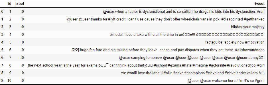
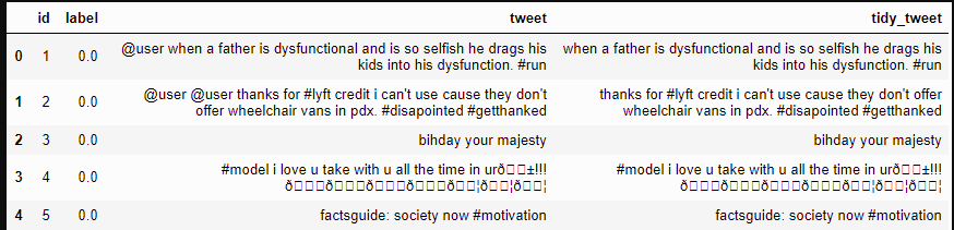
Let’s check out a few non-racist/sexist tweets.

train[train['label'] == 0].head(10)

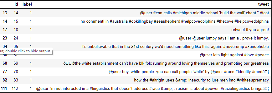
Now check out a few racist/sexist tweets.

train[train['label'] == 1].head(10)

There are quite many words and characters which are not really required. So, we will try to keep only those words that are important and add value.

Let’s check the dimensions of the train and test dataset.

train.shape, test.shape

The output is :- ((31962, 3), (17197, 2))

The train set has 31,962 tweets and the test set has 17,197 tweets.

Let’s have a glimpse at label distribution in the training dataset.

train["label"].value_counts()

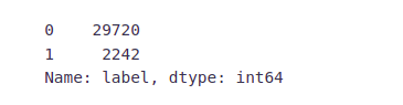
In the training dataset, we have 2,242 (~7%) tweets labeled as racist or sexist, and 29,720 (~93%) tweets labeled as non-racist/sexist. So, it is an imbalanced classification challenge.

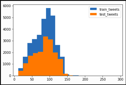
Now we will check the distribution of length of the tweets, in terms of words, in both train and test data.

length_train = train['tweet'].str.len() 
length_test = test['tweet'].str.len() 
plt.hist(length_train, bins=20, label="train_tweets") 
plt.hist(length_test, bins=20, label="test_tweets") 
plt.legend() 
plt.show()

Data Cleaning

In any natural language processing task, cleaning raw text data is an important step. It helps in getting rid of unwanted words and characters which helps in obtaining better features. If we skip this step then there is a higher chance that you are working with noisy and inconsistent data. The objective of this step is to clean noise those are less relevant to find the sentiment of tweets such as punctuation, special characters, numbers, and terms that don’t carry much weightage in context to the text.

Before we begin cleaning, let’s first combine train and test datasets. Combining the datasets will make it convenient for us to preprocess the data. Later we will split it back into train and test data.

combi = train.append(test, ignore_index=True) 
combi.shape

The output is:- (49159, 3)

Given below is a user-defined function to remove unwanted text patterns from the tweets.

def remove_pattern(input_txt, pattern):

    r = re.findall(pattern, input_txt)

    for i in r:

        input_txt = re.sub(i, '', input_txt)

    return input_txt

We will be following the steps below to clean the raw tweets in our data.

1. We will remove the Twitter handles as they are already masked as @user due to privacy concerns. These Twitter handles hardly give any information about the nature of the tweet.
2. We will also get rid of the punctuations, numbers, and even special characters since they wouldn’t help in differentiating different types of tweets.
3. Most of the smaller words do not add much value. For example, ‘pdx’, ‘his’, ‘all’. So, we will try to remove them as well from our data.
4. Lastly, we will normalize the text data. For example, reducing terms like loves, loving, and lovable to their base word, i.e., ‘love’.are often used in the same context. If we can reduce them to their root word, which is ‘love’. It will help in reducing the total number of unique words in our data without losing a significant amount of information.

1. Removing Twitter Handles (@user)

Let’s create a new column tidy_tweet, it will contain the cleaned and processed tweets. Note that we have passed “@[]*” as the pattern to the remove_pattern function. It is a regular expression that picks any word starting with ‘@’.

combi['tidy_tweet'] = np.vectorize(remove_pattern)(combi['tweet'], "@[w]*") 
combi.head()

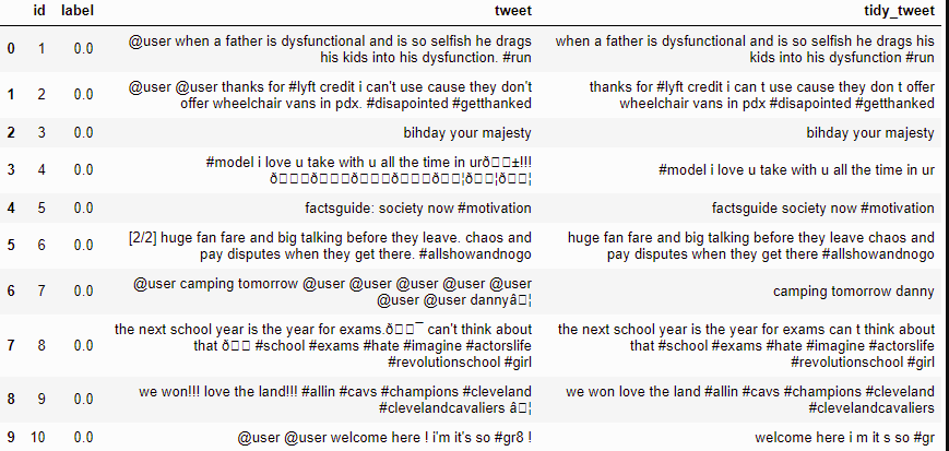
2. Removing Punctuations, Numbers, and Special Characters

Here we will replace everything except characters and hashtags with spaces. The regular expression “[^a-zA-Z#]” means anything except alphabets and ‘#’.

combi['tidy_tweet'] = combi['tidy_tweet'].str.replace("[^a-zA-Z#]", " ") 
combi.head(10)

3. Removing Short Words

We have to be a little careful here in selecting the length of the words which we want to remove. So, I have decided to remove all the words having a length of 3 or less. For example, terms like “hmm”, and “oh” are of very little use. It is better to get rid of them.

combi['tidy_tweet'] = combi['tidy_tweet'].apply(lambda x: ' '.join([w 
                        for w in x.split() if len(w)>3]))

Let’s take another look at the first few rows of the combined dataframe.

combi.head()

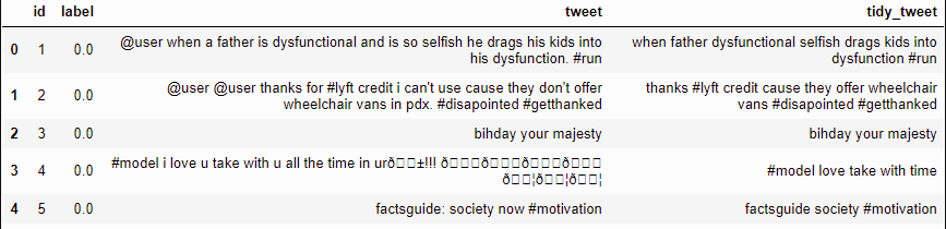
You can see the difference between the raw tweets and the cleaned tweets (tidy_tweet) quite clearly. Only the important words in the tweets have been retained and the noise (numbers, punctuations, and special characters) has been removed.

4. Text Normalization

Here we will use nltk’s PorterStemmer() function to normalize the tweets. But before that, we will have to tokenize the tweets. Tokens are individual terms or words, and tokenization is the process of splitting a string of text into tokens.

tokenized_tweet = combi['tidy_tweet'].apply(lambda x: x.split()) # tokenizing 
tokenized_tweet.head()

0 [when, father, dysfunctional, selfish, drags, kids, into, dysfunction, #run]

1 [thanks, #lyft, credit, cause, they, offer, wheelchair, vans, # disappointed, #getthanked]

2 [bihday, your, majesty]

Now we can normalize the tokenized tweets.

from nltk.stem.porter import *

stemmer = PorterStemmer() 
tokenized_tweet = tokenized_tweet.apply(lambda x: [stemmer.stem(i) for i in x])

Now let’s stitch these tokens back together. It can easily be done using nltk’s MosesDetokenizer function.

for i in range(len(tokenized_tweet)):
    tokenized_tweet[i] = ' '.join(tokenized_tweet[i]) 
combi['tidy_tweet'] = tokenized_tweet

Extracting Features from Cleaned Tweets

Bag-of-words Features

To analyze preprocessed data, it needs to be converted into features. Depending upon the usage, text features can be constructed using assorted techniques – Bag of Words, TF-IDF, and Word Embeddings. Read on to understand these techniques in detail.

from sklearn.feature_extraction.text import TfidfVectorizer, CountVectorizer
                     import gensim

Let’s start with the Bag-of-Words Features.

Consider a Corpus C of D documents {d1,d2…..dD} and N unique tokens extracted out of the corpus C. The N tokens (words) will form a dictionary and the size of the bag-of-words matrix M will be given by D X N. Each row in the matrix M contains the frequency of tokens in document D(i).

Let us understand this using a simple example.

D1: He is a lazy boy. She is also lazy.

D2: Smith is a lazy person.

The dictionary created would be a list of unique tokens in the corpus =[‘He’,’ She’,’ lazy’,’ boy’,’ Smith’,’ person’]

Here, D=2, N=6

The matrix M of size 2 X 6 will be represented as –

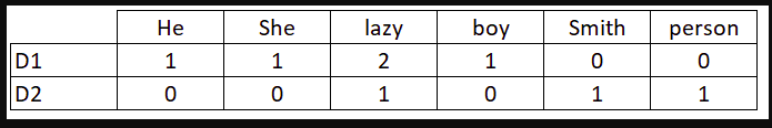
Now the columns in the above matrix can be used as features to build a classification model.

bow_vectorizer = CountVectorizer(max_df=0.90, min_df=2, max_features=1000, 
                    stop_words='english')
 bow = bow_vectorizer.fit_transform(combi['tidy_tweet']) bow.shape

TF-IDF Features

This is another method that is based on the frequency method but it is different to the bag-of-words approach in the sense that it takes into account not just the occurrence of a word in a single document (or tweet) but in the entire corpus.

TF-IDF works by penalizing the common words by assigning them lower weights while giving importance to words that are rare in the entire corpus but appear in good numbers in a few documents.

Let’s have a look at the important terms related to TF-IDF:

• TF = (Number of times term t appears in a document)/(Number of terms in the document)
• IDF = log(N/n), where, N is the number of documents and n is the number of documents a term t has appeared in.
• TF-IDF = TF*IDF

tfidf_vectorizer = TfidfVectorizer(max_df=0.90, min_df=2, max_features=1000,
                     stop_words='english') 
tfidf = tfidf_vectorizer.fit_transform(combi['tidy_tweet']) tfidf.shape

Word2Vec Features

Word embeddings are the modern way of representing words as vectors. The objective of word embeddings is to redefine the high dimensional word features into low dimensional feature vectors by preserving the contextual similarity in the corpus. They are able to achieve tasks like

King -man +woman = Queen, which is mind-blowing.

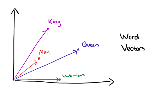
The advantages of using word embeddings over BOW or TF-IDF are:

1. Dimensionality reduction – significant reduction in the no. of features required to build a model.
2. It captures the meanings of the words, semantic relationships and the different types of contexts they are used in.

 Word2Vec Embeddings

Word2Vec is not a single algorithm but a combination of two techniques – CBOW (Continuous bag of words) Skip-gram model. Both of these are shallow neural networks that map word(s) to the target variable which is also a word(s). Both of these techniques learn weights that act as word vector representations.

CBOW tends to predict the probability of a word given a context. A context may be a single adjacent word or a group of surrounding words. The Skip-gram model works in a reverse manner, it tries to predict the context for a given word.

Below is a diagrammatic representation of a 1-word context window Word2Vec model.

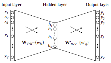
There are three layers: – an input layer, – a hidden layer, and – an output layer.

The input layer and the output, both are one- hot encoded of size [1 X V], where V is the size of the vocabulary (no. of unique words in the corpus). The output layer is a softmax layer that is used to sum the probabilities obtained in the output layer to 1. The weights learned by the model are then used as the word vectors.

We will go ahead with the Skip-gram model as it has the following advantages:

1. It can capture two semantics for a single word. i.e it will have two vector representations of ‘apple’. One for the company Apple and the other for the fruit.
2. Skip-gram with negative sub-sampling outperforms CBOW generally.

We will train a Word2Vec model on our data to obtain vector representations for all the unique words present in our corpus. There is one more option of using pre-trained word vectors instead of training our own model. Some of the freely available pre-trained vectors are:

1. Google News Word Vectors
2. Freebase names
3. DBPedia vectors (wiki2vec)

However, for this course, we will train our own word vectors since the size of the pre-trained word vectors is generally huge.

Let’s train a Word2Vec model on our corpus.

tokenized_tweet = combi['tidy_tweet'].apply(lambda x: x.split()) # tokenizing

model_w2v = gensim.models.Word2Vec(tokenized_tweet, size=200, window=5,
                min_count = 2,sg = 1,hs= 0,negative = 10,workers =2,seed= 34)

model_w2v.train(tokenized_tweet, total_examples= len(combi['tidy_tweet']), epochs=20)

Let’s play a bit with our Word2Vec model and see how it performs. We will specify a word and the model will pull out the most similar words from the corpus.

model_w2v.wv.most_similar(positive="dinner")

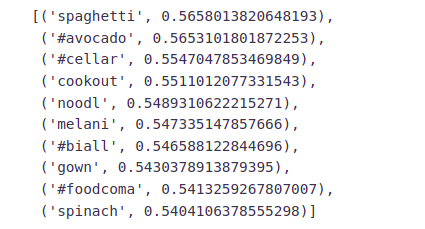
model_w2v.wv.most_similar(positive="trump")

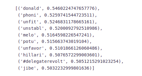
From the above two examples, we can see that our word2vec model does a good job of finding the most similar words for a given word. But how is it able to do so? That’s because it has learned vectors for every unique word in our data and it uses cosine similarity to find out the most similar vectors (words).

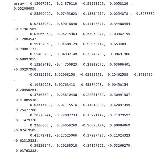
Let’s check the vector representation of any word from our corpus.

model_w2v['food']

Preparing Vectors for Tweets

Since our data contains tweets and not just words, we’ll have to figure out a way to use the word vectors from the word2vec model to create vector representation for an entire tweet. There is a simple solution to this problem, we can simply take the mean of all the word vectors present in the tweet. The length of the resultant vector will be the same, i.e. 200. We will repeat the same process for all the tweets in our data and obtain their vectors. Now we have 200 word2vec features for our data.

We will use the below function to create a vector for each tweet by taking the average of the vectors of the words present in the tweet.

def word_vector(tokens, size):
    vec = np.zeros(size).reshape((1, size))
    count =0
    for word in tokens:
        try:
        vec += model_w2v[word].reshape((1, size)
        count +=1

        except KeyError: # handling the case where the token is not in 
                            vocabulary                                     continue

     if count != 0:
        vec /= count

return vec

Preparing word2vec feature set………..

wordvec_arrays = np.zeros((len(tokenized_tweet), 200)) 
for i in range(len(tokenized_tweet)): 
   wordvec_arrays[i,:] = word_vector(tokenized_tweet[i], 200)
    wordvec_df = pd.DataFrame(wordvec_arrays) wordvec_df.shape

Now we have 200 new features, whereas in Bag of Words and TF-IDF we had 1000 features.

Model Building

We are now done with all the pre-modelling stages required to get the data in the proper form and shape. We will be building models on the datasets with different feature sets prepared in the earlier sections — Bag-of-Words, TF-IDF, word2vec vectors, and doc2vec vectors. We will use the following algorithms to build models:

1.  Logistic Regression
2.  Support Vector Machine
3.  Random Forest
4. XGBoost

Evaluation Metric

F1 score is being used as the evaluation metric. It is the weighted average of Precision and Recall. Therefore, this score takes both false positives and false negatives into account. It is suitable for uneven class distribution problems.

The important components of the F1 score are:

1. True Positives (TP) – These are the correctly predicted positive values which mean that the value of the actual class is yes and the value of the predicted class is also yes.
2. True Negatives (TN) – These are the correctly predicted negative values which mean that the value of the actual class is no and value of the predicted class is also no.
3. False Positives (FP) – When the actual class is no and the predicted class is yes.
4. False Negatives (FN) – When the actual class is yes but the predicted class is no.

Precision = TP/TP+FP

Recall = TP/TP+FN

F1 Score = 2(Recall Precision) / (Recall + Precision)

Logistic Regression

Logistic Regression is a classification algorithm. It is used to predict a binary outcome (1 / 0, Yes / No, True / False) given a set of independent variables. You can also think of logistic regression as a special case of linear regression when the outcome variable is categorical, where we are using log of odds as the dependent variable. In simple words, it predicts the probability of occurrence of an event by fitting data to a logit function.

The following equation is used in Logistic Regression:

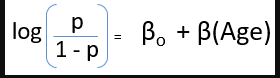
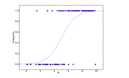
A typical logistic model plot is shown below. You can see probability never goes below 0 and above 1.

from sklearn.linear_model import LogisticRegression
 from sklearn.model_selection import train_test_split
 from sklearn.metrics import f1_score

Bag-of-Words Features

We will first try to fit the logistic regression model on the Bag-of_Words (BoW) features.

# Extracting train and test BoW features 
train_bow = bow[:31962,:] test_bow = bow[31962:,:] 
# splitting data into training and validation set
xtrain_bow, xvalid_bow, ytrain, yvalid = train_test_split(train_bow, train['label'],
                                            random_state=42,test_size=0.3)

lreg = LogisticRegression() 
# training the model lreg.fit(xtrain_bow, ytrain) 
prediction = lreg.predict_proba(xvalid_bow) # predicting on the validation set
prediction_int = prediction[:,1] >= 0.3 # if prediction is greater than or equal to 0.3 than 1 else 0 
prediction_int = prediction_int.astype(np.int) 
f1_score(yvalid, prediction_int) # calculating f1 score for the validation set

Now let’s make predictions for the test dataset and create a submission file.

test_pred = lreg.predict_proba(test_bow)
 test_pred_int = test_pred[:,1] >= 0.3 
test_pred_int = test_pred_int.astype(np.int) 
test['label'] = test_pred_int submission = test[['id','label']] 
submission.to_csv('sub_lreg_bow.csv', index=False) # writing data to a CSV file

Public Leaderboard F1 Score: 0.567

TF-IDF Features

We’ll follow the same steps as above, but now for the TF-IDF feature set.

train_tfidf = tfidf[:31962,:] 
test_tfidf = tfidf[31962:,:] 
xtrain_tfidf = train_tfidf[ytrain.index]
 xvalid_tfidf = train_tfidf[yvalid.index]

lreg.fit(xtrain_tfidf, ytrain) 
prediction = lreg.predict_proba(xvalid_tfidf)
prediction_int = prediction[:,1] >= 0.3
prediction_int = prediction_int.astype(np.int) 
f1_score(yvalid, prediction_int) # calculating f1 score for the validation set

Public Leaderboard F1 Score: 0.564

Word2Vec Features

train_w2v = wordvec_df.iloc[:31962,:] 
test_w2v = wordvec_df.iloc[31962:,:] 
xtrain_w2v = train_w2v.iloc[ytrain.index,:] 
xvalid_w2v = train_w2v.iloc[yvalid.index,:]

lreg.fit(xtrain_w2v, ytrain) 
prediction = lreg.predict_proba(xvalid_w2v) 
prediction_int = prediction[:,1] >= 0.3
prediction_int = prediction_int.astype(np.int) 
f1_score(yvalid, prediction_int)

Public Leaderboard F1 Score: 0.661

Doc2Vec Features

train_d2v = docvec_df.iloc[:31962,:] 
test_d2v = docvec_df.iloc[31962:,:] 
xtrain_d2v = train_d2v.iloc[ytrain.index,:] 
xvalid_d2v = train_d2v.iloc[yvalid.index,:]

lreg.fit(xtrain_d2v, ytrain) 
prediction = lreg.predict_proba(xvalid_d2v) 
prediction_int = prediction[:,1] >= 0.3 
prediction_int = prediction_int.astype(np.int)
 f1_score(yvalid, prediction_int)

Public Leaderboard F1 Score: 0.381

Doc2Vec features do not seem to be capturing the right signals as both the F1 scores, on the validation set and on the public leaderboard are quite low.

Support Vector Machine(SVM)

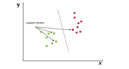
Support Vector Machine (SVM) is a supervised machine learning algorithm that can be used for both classification and regression challenges. However, it is mostly used in classification problems. In this algorithm, we plot each data item as a point in n-dimensional space (where n is the number of features you have) with the value of each feature being the value of a particular coordinate. Then, we perform classification by finding the hyper-plane that differentiates the two classes as shown in the plot below:

from sklearn import svm

Bag-of-Words Features

svc = svm.SVC(kernel='linear', C=1, probability=True).fit(xtrain_bow, ytrain) 
prediction = svc.predict_proba(xvalid_bow) 
prediction_int = prediction[:,1] >= 0.3 
prediction_int = prediction_int.astype(np.int) 
f1_score(yvalid, prediction_int)

Again let’s make predictions for the test dataset and create another submission file.

test_pred = svc.predict_proba(test_bow) 
test_pred_int = test_pred[:,1] >= 0.3 
test_pred_int = test_pred_int.astype(np.int) 
test['label'] = test_pred_int 
submission = test[['id','label']] 
submission.to_csv('sub_svm_bow.csv', index=False)

Public Leaderboard F1 Score: 0.554

Here both validation score and leaderboard score are slightly lesser than the Logistic Regression scores for bag-of-words features.

TF-IDF Features

svc = svm.SVC(kernel='linear', c=1, probability=True).fit(xtrain_tfidf, ytrain) 
prediction = svc.predict_proba(xvalid_tfidf)

prediction_int = prediction[:,1] >= 0.3

prediction_int = prediction_int.astype(np.int)

f1_score(yvalid, prediction_int)

Public Leaderboard F1 Score: 0.546

Word2Vec Features

svc = svm.SVC(kernel='linear', C=1, probability=True).fit(xtrain_w2v, ytrain) 
prediction = svc.predict_proba(xvalid_w2v)

prediction_int = prediction[:,1] >= 0.3

prediction_int = prediction_int.astype(np.int) f1_score(yvalid, prediction_int)

Public Leaderboard F1 Score: 0.654

Doc2Vec Features

svc = svm.SVC(kernel='linear', C=1, probability=True).fit(xtrain_d2v, ytrain) 
prediction = svc.predict_proba(xvalid_d2v)

prediction_int = prediction[:,1] >= 0.3 
prediction_int = prediction_int.astype(np.int) 
f1_score(yvalid, prediction_int)

Public Leaderboard F1 Score: 0.214

Random Forest

Random Forest is a versatile machine learning algorithm capable of performing both regression and classification tasks. It is a kind of ensemble learning method, where a few weak models combine to form a powerful model. In Random Forest, we grow multiple trees as opposed to a decision single tree. To classify a new object based on attributes, each tree gives a classification and we say the tree “votes” for that class. The forest chooses the classification having the most votes (over all the trees in the forest).

It works in the following manner. Each tree is planted & grown as follows:

1. Assume the number of cases in the training set is N. Then, a sample of these N cases is taken at random but with replacement. This sample will be the training set for growing the tree.
2. If there are M input variables, a number m (m<M) is specified such that at each node, m variables are selected at random out of the M. The best split on these m variables is used to split the node. The value of m is held constant while we grow the forest.
3. Each tree is grown to the largest extent possible and there is no pruning. Each tree is grown to the largest extent possible and there is no pruning.
4. Predict new data by aggregating the predictions of the ntree trees (i.e., majority votes for classification, the average for regression).

from sklearn.ensemble import RandomForestClassifier

Bag-of-Words Features

First, we will train our RandomForest model on the Bag-of-Words features and check its performance on both the validation set and public leaderboard.

rf = RandomForestClassifier(n_estimators=400, random_state=11).fit(xtrain_bow, ytrain) 
prediction = rf.predict(xvalid_bow) 
# validation score f1_score(yvalid, prediction)

Let’s make predictions for the test dataset and create another submission file.

test_pred = rf.predict(test_bow) test['label'] = test_pred 
submission = test[['id','label']]
submission.to_csv('sub_rf_bow.csv', index=False)

Public Leaderboard F1 Score: 0.598.

TF-IDF Features

rf =RandomForestClassifier(n_estimators=400, random_state=11).fit(xtrain_tfidf, ytrain) 
prediction = rf.predict(xvalid_tfidf)
f1_score(yvalid, prediction)

Public Leaderboard F1 Score: 0.589.

Word2Vec Features

rf = RandomForestClassifier(n_estimators=400, random_state=11).fit(xtrain_w2v, ytrain) 
prediction = rf.predict(xvalid_w2v) 
f1_score(yvalid, prediction)

Public Leaderboard F1 Score: 0.549

Doc2Vec Features

rf = RandomForestClassifier(n_estimators=400, random_state=11).fit(xtrain_d2v, ytrain) 
prediction = rf.predict(xvalid_d2v) 
f1_score(yvalid, prediction)

Public Leaderboard F1 Score: 0.07.

XGBoost

Extreme Gradient Boosting (xgboost) is an advanced implementation of a gradient boosting algorithm. It has both linear model solver and tree learning algorithms. Its ability to do parallel computation on a single machine makes it extremely fast. It also has additional features for cross-validation and finding important variables. There are many parameters that need to be controlled to optimize the model.

Some key benefits of XGBoost are:

1. Regularization:- – helps in reducing overfitting
2. Parallel Processing:- – XGBoost implements parallel processing and is blazingly faster as compared to GBM.
3. Handling Missing Values:- – It has an in-built routine to handle missing values.
4. Built-in Cross-Validation:- allows user to run cross-validation at each iteration of the boosting process

from xgboost import XGBClassifier

Bag-of-Words Features

xgb_model = XGBClassifier(max_depth=6, n_estimators=1000).fit(xtrain_bow, ytrain) 
prediction = xgb_model.predict(xvalid_bow) f1_score(yvalid, prediction)

test_pred = xgb_model.predict(test_bow) test['label'] = test_pred
 submission = test[['id','label']] 
submission.to_csv('sub_xgb_bow.csv', index=False)

Public Leaderboard F1 Score: 0.554.

TF-IDF Features

xgb = XGBClassifier(max_depth=6, n_estimators=1000).fit(xtrain_tfidf, ytrain) 
prediction = xgb.predict(xvalid_tfidf) f1_score(yvalid, prediction)

Public Leaderboard F1 Score: 0.554

Word2Vec Features

xgb = XGBClassifier(max_depth=6, n_estimators=1000, nthread= 3).fit(xtrain_w2v, ytrain) 
prediction = xgb.predict(xvalid_w2v) f1_score(yvalid, prediction)

Public Leaderboard F1 Score: 0.698

XGBoost model on word2vec features has outperformed all the previous models in this course.

Doc2Vec Features

xgb = XGBClassifier(max_depth=6, n_estimators=1000, nthread= 3).fit(xtrain_d2v, ytrain) 
prediction = xgb.predict(xvalid_d2v) f1_score(yvalid, prediction)

Public Leaderboard F1 Score: 0.374

Conclusion to Sentiment Analysis

Now it’s time to wrap up things. Let’s quickly revisit what we have learned in this course, initially we cleaned our raw text data, then we learned about 4 different types of feature-set that we can extract from any text data, and finally we used this feature sets to build models for sentiment analysis. Below is a summary table showing F1 scores for different models and feature sets.

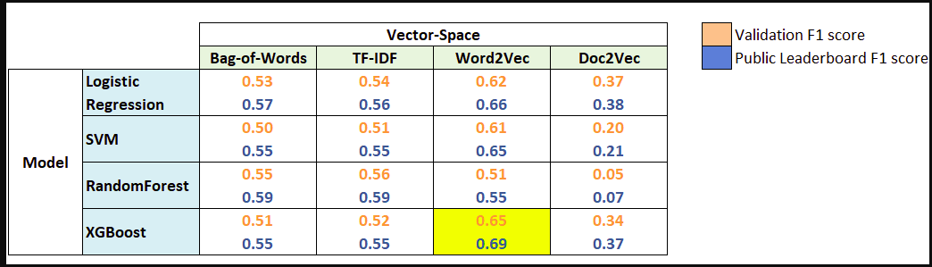
Word2Vec features turned out to be most useful. Whereas XGBoost with Word2Vec features was the best model for this problem. This clearly shows the power of word embeddings in dealing with NLP problems.

What else can be tried?

We have covered a lot in this Sentiment Analysis course, but still, there is plenty of room for other things to try out. Given below is a list of tasks that you can try with this data.

1. We have built so many models in this course, that we can definitely try model ensembling. A simple ensemble of all the submission files (maximum voting) yielded an F1 score of 0.55 on the public leaderboard.
2. Use Parts-of-Speech tagging to create new features.
3. Use stemming and/or lemmatization. It might help in getting rid of unnecessary words.
4. Use bi-grams or tri-grams (tokens of 2 or 3 words respectively) for Bag-of-Words and TF-IDF.
5. We can give pre-trained word-embeddings models a try.