Introduction
In the world of artificial intelligence, generative AI, data science, and machine learning, the Naive Bayes classifier is a fundamental probabilistic classifier built upon Bayes’ theorem. Known for its simplicity and effectiveness, this algorithm is precious for text classification tasks such as spam filtering and sentiment analysis. This tutorial will explore building a Naive Bayesian classifier from scratch using Python. We will explore the mechanics of Bayes’ theorem, understand how to handle conditional probabilities and apply Laplace smoothing to manage unseen words in our dataset. We will preprocess the IMDB movie reviews dataset through a hands-on approach, encode text data into numerical features, and ultimately construct a robust sentiment analysis model. You will clearly understand how to implement and utilize the sentiment analysis using Naive Bayes Classifier.
Learning Outcomes
- Gain a comprehensive understanding of the Naive Bayes classifier, its foundational basis in Bayes’ theorem, and its application as a probabilistic classification algorithm in sentiment analysis.
- Learn to construct a Naive Bayes classifier without relying on machine learning libraries.
- Develop skills in preprocessing text data for sentiment analysis, including techniques such as removing HTML tags and URLs.
- Acquire the ability to implement and evaluate a Naive Bayes classifier on a real dataset (e.g., IMDB movie reviews) by splitting data into training and test sets, fitting the model, making predictions, and calculating accuracy metrics.
This article was published as a part of the Data Science Blogathon.
Table of contents
What is a Naive Bayes Classifier?
The Naive Bayes algorithm is a supervised machine learning algorithm based on the Bayes theorem. It is a probabilistic classifier often used in NLP tasks like sentiment analysis (identifying a text corpus’ emotional or sentimental tone or opinion).
The Bayes’ theorem is used to determine the probability of a hypothesis when prior knowledge is available. It depends on conditional probabilities.
How Does Naive Bayes Classifier Work?
Let’s see how a Naive Bayes classifier works.
The formula for conditional probabilities is given below :
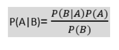
P(A|B) is the posterior probability, i.e., the probability of a hypothesis A, given that event B occurs. P(B|A) is likelihood probability, i.e., the probability of the evidence given that hypothesis A is true. P(A) is prior probability, i.e., the probability of the hypothesis before observing the evidence, and P(B) is marginal, i.e., the probability of the evidence. When Bayes’ theorem is applied to classify text documents, the class variable c of a particular document d is given by :
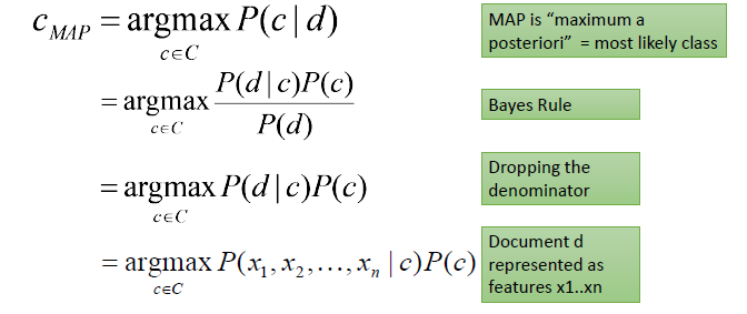
Let the feature conditional probabilities P(x_i | c) be independent of each other (conditional independence assumption). So,
P(x_1, x_2, …, x_n | c) = P(x_1 | c) X P(x_2 | c) X … X P(x_n | c)
Now, if we consider words as the features of the document, the individual feature conditional probabilities can be calculated using the following formula :
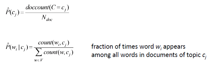
But what if a given word w_i does not occur in any training document of class c_j but appears in a text document? P(w_i | c_j) will become 0, which means the probability of the test document belonging to class c_j will become 0. To avoid this, Laplace smoothing is introduced, and the conditional feature probabilities are calculated in the following way :
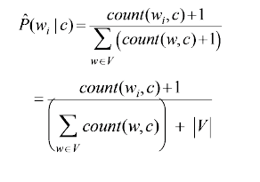
where |V| is the number of unique words in the text corpus. This way we can easily deal with unseen test words.
Types of Naive Bayes Model
There are three types of Naive Bayes model
Multinomial Naive Bayes
Multinomial Naive Bayes is used for discrete data, particularly in text classification. This model assumes that features represent the frequencies or counts of discrete events, such as word counts in documents. It is widely applied in document classification, spam detection, and sentiment analysis, where the occurrence and frequency of words are critical indicators.
Bernoulli Naive Bayes
Bernoulli Naive Bayes is designed for binary or boolean features. It assumes that features are binary, indicating the presence or absence of a word in a document. This model is particularly effective for document classification tasks that use binary term occurrence features and for spam detection, where the binary presence of specific keywords can determine the classification.
Gaussian Naive Bayes
Gaussian Naive Bayes is suitable for continuous data. It assumes that the features follow a Gaussian (normal) distribution. This model is often applied in scenarios involving continuous input variables, such as medical diagnosis and financial analysis, predicting outcomes based on continuous attributes like patient metrics or financial indicators.
Advantages of Naive Bayes Classifier
- Simplicity and Speed: The Naive Bayes classifier is straightforward to implement using Python libraries, making it an ideal choice for beginners in data science and artificial intelligence. Due to its simplicity requires less training data and computational resources compared to more complex machine learning algorithms like neural networks and logistic regression.
- Effective with Small Datasets: The Naive Bayes classifier performs well even with small training datasets. This is particularly useful when collecting large amounts of labeled data is challenging.
- Efficient for High-Dimensional Data: The Naive Bayes algorithm efficiently handles high-dimensional data. It works well with text classification tasks, such as spam filtering and sentiment analysis, where feature vectors can be very large.
- Robust to Irrelevant Features: The model is less sensitive to irrelevant features because it calculates the conditional probability for each feature independently. This robustness helps maintain good performance even with noisy data.
- Less Prone to Overfitting: Naive Bayes classifiers are less prone to overfitting, especially compared to more complex models. This characteristic is beneficial for generalizing well on unseen test datasets.
- Interpretability: The Naive Bayes model’s probabilistic nature makes it easy to understand and interpret. Users can see the influence of individual predictors on the final classification.
Disadvantages of Naive Bayes Classifier
- Independence Assumption: The core limitation of the Naive Bayes classifier is the independence assumption. In many real-world datasets, predictors are often correlated, violating this assumption and potentially reducing model accuracy.
- Zero Probability Problem: If a feature value in the test dataset was not present in the training dataset, the model assigns a zero probability to the posterior probability, leading to issues in classification. Techniques like Laplace smoothing can mitigate this but do not completely solve the problem.
- Performance with Complex Relationships: Naive Bayes models may struggle with datasets where feature interactions significantly impact the class labels. In such cases, models that capture these interactions, like decision trees or neural networks, may perform better.
- Limited by Gaussian Assumption: When using Gaussian Naive Bayes, the assumption that continuous features follow a normal distribution may not always hold, limiting its applicability for certain datasets.
- Binary/Bernoulli Limitation: The model assumes binary feature values for Bernoulli Naive Bayes, which may not capture the complexity of datasets with more nuanced feature representations.
Also Read: Conditional Probability and Bayes theorem in R
What is Sentiment Analysis?
Sentiment analysis, also known as opinion mining, is a subfield of natural language processing (NLP) that focuses on determining the emotional tone behind a body of text. This analysis aims to identify and extract subjective information from textual data, such as attitudes, opinions, and emotions. The goal is to classify the polarity of the text, whether it is positive, negative, or neutral, and sometimes to identify more nuanced emotional states.
How to Build a Naive Bayes Classifier?
Loading the Dataset
We will perform sentiment analysis on the IMDB dataset, which has 25k positive and 25k negative movie reviews. We need to build an NB classifier that classifies an unseen movie review as positive or negative. The dataset can be downloaded from here. Let us start by importing the necessary packages for text manipulation and loading the dataset into a pandas dataframe :
import re

import pandas as pd

import numpy as np

from sklearn.preprocessing import LabelEncoder

from sklearn.model_selection import train_test_split

from sklearn.metrics import classification_report

from sklearn.metrics import accuracy_score

import math

import nltk

from sklearn.feature_extraction.text import CountVectorizer

from collections import defaultdict

data = pd.read_csv('IMDB Dataset.csv')

data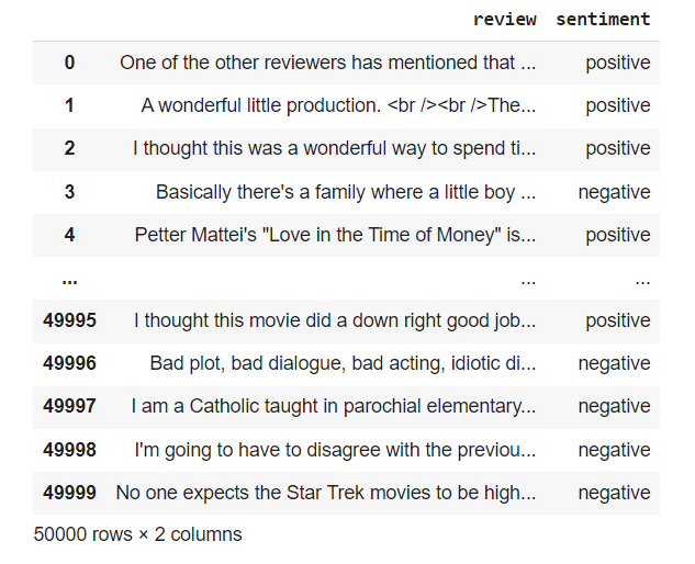
Data Preprocessing
Using regex functions, we remove HTML tags, URLs, and non-alphanumeric characters from the dataset. Stopwords (commonly used words like ‘and,’ ‘the,’ and ‘at’ that do not hold any special meaning in a sentence) are also removed from the corpus using the nltk stopwords list :
def remove_tags(string):
    removelist = ""
    result = re.sub('','',string)          #remove HTML tags
    result = re.sub('https://.*','',result)   #remove URLs
    result = re.sub(r'[^w'+removelist+']', ' ',result)    #remove non-alphanumeric characters
    result = result.lower()
    return result
data['review']=data['review'].apply(lambda cw : remove_tags(cw))
nltk.download('stopwords')
from nltk.corpus import stopwords
stop_words = set(stopwords.words('english'))
data['review'] = data['review'].apply(lambda x: ' '.join([word for word in x.split() if word not in (stop_words)]))
Finally, we perform lemmatization on the text. Lemmatization is used to find the root form of words or lemmas in NLP. For example, the lemma of the words reading, reads, read is read. This helps save unnecessary computational overhead in deciphering entire words since most words’ meanings are well-expressed by their separate lemmas. We perform lemmatization using the WordNetLemmatizer() from nltk. The text is first broken into individual tokens/ words using the WhitespaceTokenizer() from nltk. We write a function lemmatize_text to perform lemmatization on the individual words.
Also Read: Stemming vs Lemmatization in NLP: Must-Know Differences
w_tokenizer = nltk.tokenize.WhitespaceTokenizer()
lemmatizer = nltk.stem.WordNetLemmatizer()
def lemmatize_text(text):
st = ""
for w in w_tokenizer.tokenize(text):
st = st + lemmatizer.lemmatize(w) + " "
return st
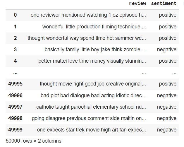
data['review'] = data.review.apply(lemmatize_text)The dataset looks like this after preprocessing :
Encoding Labels and Making Train-Test Splits
LabelEncoder() from sklearn.preprocessing is used to convert the labels (‘positive’, ‘negative’) into 1’s and 0’s respectively.
reviews = data['review'].values
labels = data['sentiment'].values
encoder = LabelEncoder()
encoded_labels = encoder.fit_transform(labels)
The dataset is then split into 80% train and 20% test parts using train_test_split from sklearn.model_selection.
train_sentences, test_sentences, train_labels, test_labels = train_test_split(reviews, encoded_labels, stratify = encoded_labels)Using Formulas
Many variants of the Naive Bayes classification are available in the scikit-learn library. However, we will build our classifier using the formulas described earlier. We start using the CountVectorizer from sklearn.feature_extraction.text to get the frequency of each word appearing in the training set. We store them in a dictionary called ‘word_counts’. All the unique words in the corpus are stored in ‘vocab.’
vec = CountVectorizer(max_features = 3000)
X = vec.fit_transform(train_sentences)
vocab = vec.get_feature_names()
X = X.toarray()
word_counts = {}
for l in range(2):
    word_counts[l] = defaultdict(lambda: 0)
for i in range(X.shape[0]):
    l = train_labels[i]
    for j in range(len(vocab)):
        word_counts[l][vocab[j]] += X[i][j]
As we mentioned earlier, we need to perform Laplace smoothing to handle words in the test set that are absent in the training set. We define a function ‘laplace_smoothing’, which takes the vocabulary and the raw ‘word_counts’ dictionary and returns the smoothened conditional probabilities.
def laplace_smoothing(n_label_items, vocab, word_counts, word, text_label):
    a = word_counts[text_label][word] + 1
    b = n_label_items[text_label] + len(vocab)
    return math.log(a/b)
We define the ‘fit’ and ‘predict’ functions for our classifier.
def group_by_label(x, y, labels):
    data = {}
    for l in labels:
        data[l] = x[np.where(y == l)]
    return data
def fit(x, y, labels):
n_label_items = {}
log_label_priors = {}
n = len(x)
grouped_data = group_by_label(x, y, labels)
for l, data in grouped_data.items():
n_label_items[l] = len(data)
log_label_priors[l] = math.log(n_label_items[l] / n)
return n_label_items, log_label_priorsThe ‘fit’ function takes x (reviews) and y (labels – ‘positive,’ ‘negative’) values to be fitted on and returns the number of reviews with each label and the apriori conditional probabilities. Finally, the ‘predict’ function is written, which returns predictions on unseen test reviews.
def predict(n_label_items, vocab, word_counts, log_label_priors, labels, x):
    result = []
    for text in x:
        label_scores = {l: log_label_priors[l] for l in labels}
        words = set(w_tokenizer.tokenize(text))
        for word in words:
            if word not in vocab: continue
            for l in labels:
                log_w_given_l = laplace_smoothing(n_label_items, vocab, word_counts, word, l)
                label_scores[l] += log_w_given_l
        result.append(max(label_scores, key=label_scores.get))
    return result
Fitting the Model on Training Set and Evaluating Accuracies on the Test Set
The classifier is now fitted on the train_sentences and used to predict labels for the test_sentences. The prediction accuracy on the test set is 85.16%, which is pretty good. We calculate accuracy using ‘accuracy_score’ from sklearn.metrics.
labels = [0,1]
n_label_items, log_label_priors = fit(train_sentences,train_labels,labels)
pred = predict(n_label_items, vocab, word_counts, log_label_priors, labels, test_sentences)
print("Accuracy of prediction on test set : ", accuracy_score(test_labels,pred))
How is Naive Bayes Used in Sentiment Analysis?
Sentiment analysis with the Naive Bayesian model is a common technique for classifying text data as positive, negative, or neutral. Here’s a breakdown of how it works:
Data Preparation:
In sentiment analysis, a text data collection is labeled as positive, negative, or neutral, forming the training dataset. This data is then preprocessed to clean and standardize the text, which may involve removing punctuation, converting text to lowercase, and other tasks.
Feature Engineering:
Each text data point is represented as a “bag of words,” where each feature represents the presence or absence of a particular word in the text. This step involves creating a numerical representation of the text data, making it suitable for machine learning algorithms like Naive Bayes.
Model Training:
The Naive Bayes classifier learns the probability of each word appearing in positive, negative, or neutral text from the training data. It calculates the conditional probabilities of words given each sentiment class. Also, the Naive Bayes classification can be evaluated by plotting a confusion matrix.
Sentiment Prediction:
When given a new text, the trained Naive Bayes model calculates the probability of each word belonging to each sentiment class. Bayes’ theorem combines these probabilities to predict the sentiment class label with the highest overall probability.
Advantages of Naive Bayes Classifier for Sentiment Analysis
- The Naive Bayes classifier is straightforward to implement using popular Python libraries such as scikit-learn. This machine learning algorithm requires minimal computation, making it suitable for large datasets and real-time applications. The naive Bayes algorithm simplifies the computation of posterior probabilities by leveraging the Bayes theorem and assuming conditional independence of features. This makes the model fast and efficient for classification tasks.
- The Naive Bayes classifier can perform well even with relatively small training data. This is particularly beneficial in scenarios where collecting large labeled datasets is challenging. For sentiment analysis, where the amount of annotated text can be limited, multinomial naive Bayes or Bernoulli naive Bayes models can still deliver robust results.
- The Naive Bayes model provides an intuitive way to interpret results by showing the influence of individual words (or predictors) on the final classification. Given a class label, each word’s contribution can be understood in conditional probability. This transparency is beneficial in text classification problems like sentiment analysis, where understanding why a particular sentiment is assigned can be as important as the classification itself.
Limitations of Naive Bayes Classifier for Sentiment Analysis
- The Naive Bayes classifier makes a strong independence assumption that features (words, in the case of text) are independent given the class label. In natural language, however, words often appear in contextually dependent sequences. This assumption can lead to inaccuracies in sentiment analysis, where the relationships between words (e.g., negations, phrases) are crucial for correctly understanding the sentiment.
- The Naive Bayes model can be overly sensitive to rare or absent words from the training dataset. If a word in the test dataset has never been seen before, the model might assign it a probability of zero, which can skew the classification. Techniques like Laplace smoothing can mitigate this issue, but they don’t entirely solve the problem of handling rare or unseen feature values. This sensitivity can impact the model’s performance on real-world sentiment analysis tasks, where new words and phrases regularly emerge.
Conclusion
In conclusion, building a Naive Bayes classifier from scratch for sentiment analysis involves understanding the fundamentals of Bayes’ theorem and implementing conditional probabilities. Through hands-on preprocessing of text data, including removing HTML tags, URLs, and stopwords, we prepare the IMDB movie reviews dataset for analysis. We construct our Naive Bayes classifier, considering three types: Multinomial NB, Bernoulli Naive Bayes, and Gaussian NB, each suitable for different data types. Despite its simplicity, Naive Bayes offers advantages such as speed, efficiency with small datasets, and robustness to irrelevant features. However, it has limitations like the independence assumption and sensitivity to rare words. Overall, this tutorial equips readers with the skills to effectively implement and evaluate Naive Bayes classifiers for sentiment analysis tasks.
The key takeaways from this article are :
- A Naive Bayes classifier is a probabilistic ML classifier based on the Bayes theorem.
- We can build our own NB classifier from scratch for text classification, such as sentiment analysis or spam filtering.
- Laplace smoothing needs to be performed while calculating feature conditional probabilities so that we can handle unseen test words not present in the training corpus.
If you want to learn more about Artificial Intelligence, Machine learning models, supervised learning, and Generative AI, follow Analytics Vidhya’s blog.
The media shown in this article is not owned by Analytics Vidhya and are used at the Author’s discretion.
Frequently Asked Questions
Q1. How is Naive Bayes used in sentiment analysis?
A. In sentiment analysis, Naive Bayes is utilized to classify text sentiment. The approach assumes features (words) are independent given the sentiment. It calculates the probability of a text belonging to each sentiment class based on word frequencies. Then, it assigns the class with the highest probability. Despite its simplicity, Naive Bayes often performs well in sentiment analysis by quickly capturing word patterns associated with different sentiments.
Q2. Which algorithm is used for sentiment analysis?
A. Sentiment analysis tools use different tricks to understand feelings in text:
Simple list: Checks for happy or sad words but misses sarcasm and new words.
Learns from examples: Needs a lot of training data but works better than a list.
Super learner (complex): Most powerful, but needs a lot of computer power.pen_spark
Q3. Is Naive Bayes a classifier or a regression?
A. Naive Bayes is a classifier. It classifies data into distinct categories based on probabilistic calculations derived from Bayes’ theorem.
Q4.What are the 3 different Naive Bayes classifiers?
A. The three different Naive Bayes classifiers are:
Multinomial Naive Bayes: Used for discrete data, especially word counts in text classification.
Bernoulli Naive Bayes: Used for binary/boolean features.
Gaussian Naive Bayes: Used for continuous data, assuming a Gaussian distribution.
Q5. What is an example of a Naive Bayes problem?
A. An example of a Naive Bayes problem is sentiment analysis, where the goal is to classify text (such as movie reviews) as positive or negative based on the words used in the text.
Q6. Why is it called Naive Bayes?
A. It is called “Naive Bayes” because it makes a naive assumption that all features are independent of each other given the class label, which simplifies the computation of probabilities.