This article was published as a part of the Data Science Blogathon.
About the Competition
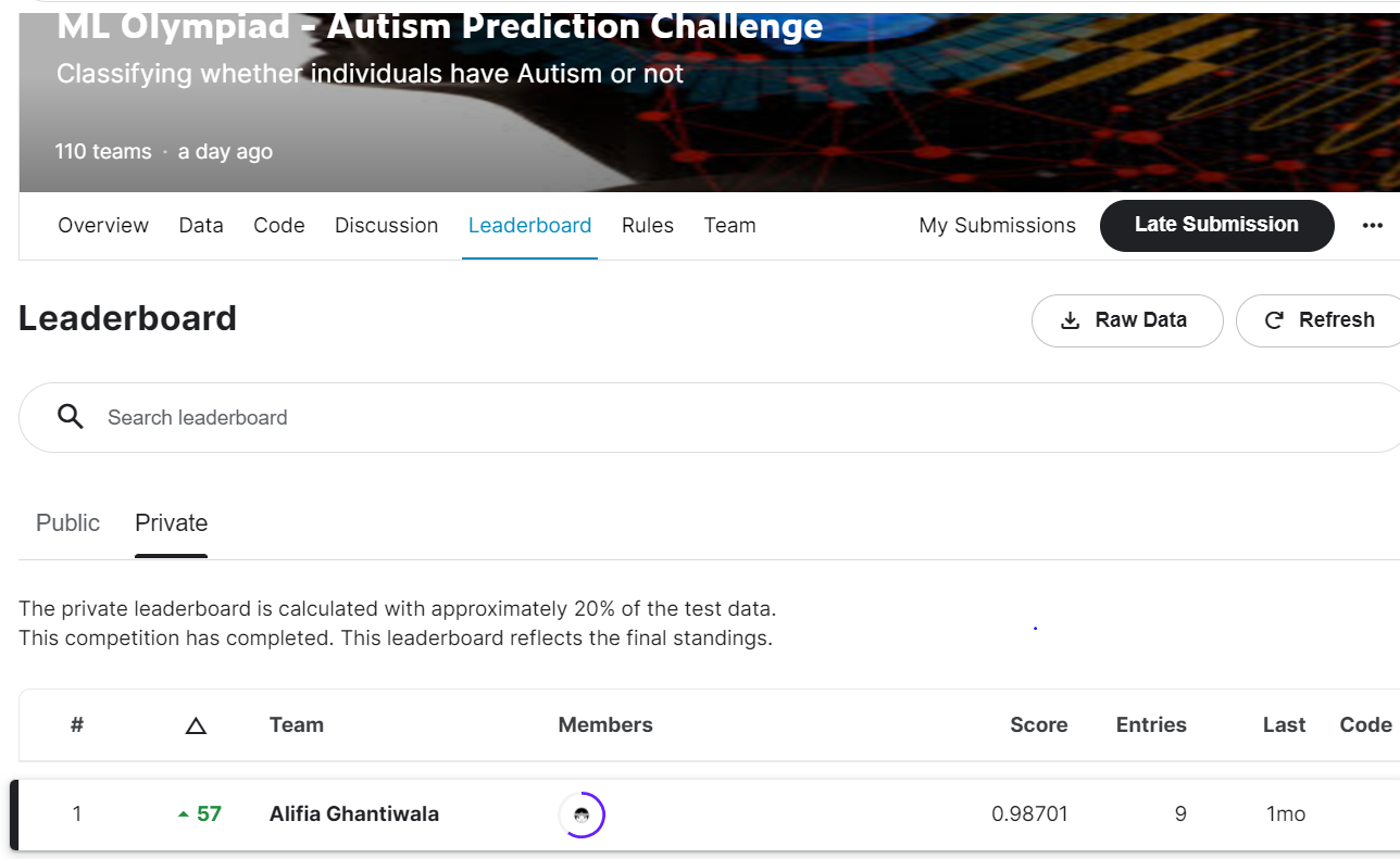
The competition was to predict the likelihood of having Autism. It was sponsored by Google Developers and hosted on Kaggle. The data was collected from people that filled out an app form. Research has proven that early detection of autism can help in incrementing mental development, communication, and social skills. This was the main driving force of the challenge, to provide an automated and reliable solution to healthcare workers so that they can prioritize their resources.
The Approach I Followed to Win the Competition
0) Understanding the data
1) Using label encoder to encode categorical features
2) Removal of features based on their correlation with the target
3) Using Grid Search and 5 fold cross-validation for hyperparameter optimization.
4) For modelling, I used XGBoost and LightGBM and combined their results based on CV performance.
Understanding the Data
Understanding the data would be our first step. The most powerful machine learning model would not produce desired results with garbage input. I did a univariate and bivariate analysis to understand the input completely, based on the same, I did feature selection.
Features in our dataset
ID – ID of the patient
A1_Score to A10_Score – Score based on Autism Spectrum Quotient (AQ)
age – Patient’s age in years
gender – Gender of the patient
ethnicity – Ethnicity of the patient
jaundice – Whether the person was having jaundice at birth
autism – If an immediate family member was diagnosed with autism
contry_of_res – Country of patient
used_app_before – If a person has undergone a screening test
result – Score for AQ1-10 screening test
age_desc – Age of the patient
relation – Relation of a patient who completed the test
Class/ASD – Target label
train.columns
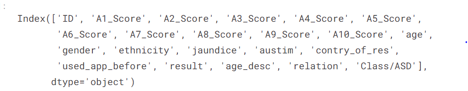
Source: Author
Univariate Analysis
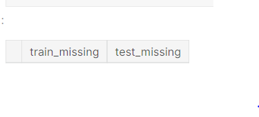
ncounts = pd.<a onclick="parent.postMessage({'referent':'.pandas.DataFrame'}, '*')">DataFrame([train.isna().mean(), test.isna().mean()]).T
ncounts = ncounts.rename(columns={0: "train_missing", 1: "test_missing"})

ncounts.query("train_missing > 0")
Source: Author
The input data does not have NA values.
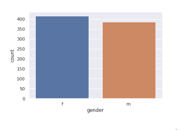
Gender feature
sns.<a onclick="parent.postMessage({'referent':'.seaborn.set_theme'}, '*')">set_theme(style="darkgrid")
sns.<a onclick="parent.postMessage({'referent':'.seaborn.countplot'}, '*')">countplot(x='gender',data=train)
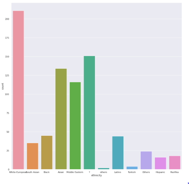
Ethnicity
plt.<a onclick="parent.postMessage({'referent':'.matplotlib.pyplot.figure'}, '*')">figure(figsize=(15,15))
sns.<a onclick="parent.postMessage({'referent':'.seaborn.countplot'}, '*')">countplot(x='ethnicity',data=train)
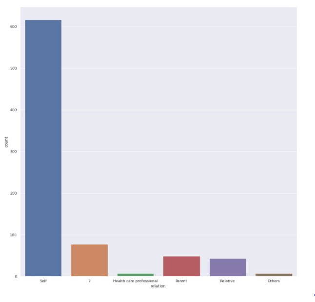
Relation feature
sns.<a onclick="parent.postMessage({'referent':'.seaborn.set_theme'}, '*')">set_theme(style="darkgrid")
plt.<a onclick="parent.postMessage({'referent':'.matplotlib.pyplot.figure'}, '*')">figure(figsize=(15,15))
sns.<a onclick="parent.postMessage({'referent':'.seaborn.countplot'}, '*')">countplot(x='relation',data=train)
Age feature
sns.<a onclick="parent.postMessage({'referent':'.seaborn.set_theme'}, '*')">set_theme(style="darkgrid")
plt.<a onclick="parent.postMessage({'referent':'.matplotlib.pyplot.figure'}, '*')">figure(figsize=(15,15))
sns.<a onclick="parent.postMessage({'referent':'.seaborn.countplot'}, '*')">countplot(x='age_desc',data=train)
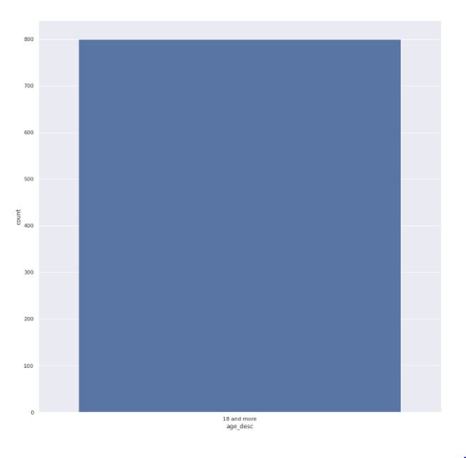
We have 800 different age values but all of them are older than 800
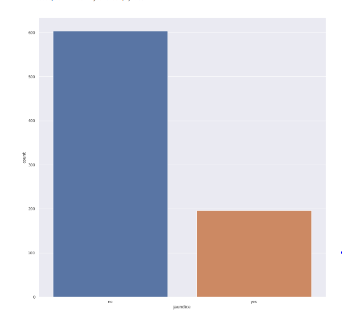
Jaundice feature
sns.<a onclick="parent.postMessage({'referent':'.seaborn.set_theme'}, '*')">set_theme(style="darkgrid")
plt.<a onclick="parent.postMessage({'referent':'.matplotlib.pyplot.figure'}, '*')">figure(figsize=(15,15))
sns.<a onclick="parent.postMessage({'referent':'.seaborn.countplot'}, '*')">countplot(x='jaundice',data=train)
Autism feature
sns.<a onclick="parent.postMessage({'referent':'.seaborn.set_theme'}, '*')">set_theme(style="darkgrid")
plt.<a onclick="parent.postMessage({'referent':'.matplotlib.pyplot.figure'}, '*')">figure(figsize=(15,15))
sns.<a onclick="parent.postMessage({'referent':'.seaborn.countplot'}, '*')">countplot(x='austim',data=train)

Country of patient feature
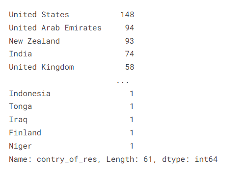
train["contry_of_res"].value_counts()
A1 to A10 score feature
score_columns = ["A1_Score","A2_Score","A3_Score","A4_Score","A5_Score","A6_Score","A7_Score","A8_Score","A9_Score","A10_Score"]
i = 1
for col in score_columns:
    plt.<a onclick="parent.postMessage({'referent':'.matplotlib.pyplot.figure'}, '*')">figure(figsize=(10,15))
    plt.<a onclick="parent.postMessage({'referent':'.matplotlib.pyplot.subplot'}, '*')">subplot(10,1,i)
    sns.<a onclick="parent.postMessage({'referent':'.seaborn.countplot'}, '*')">countplot(train[col])
    i += 1
Result (target feature)
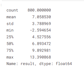
train["result"].describe()
sns.<a onclick="parent.postMessage({'referent':'.seaborn.scatterplot'}, '*')">scatterplot(data=train,x="result",y="Class/ASD")
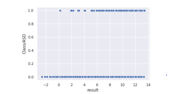
Observation: Result values less than 0 are only class 0 target
Insights from Univariate Analysis
-
No missing/NA data
- No columns with constant values
- Gender distribution in the train and test datasets is the same and is balanced.
- The highest number of patients are from ethnicity ‘White European’ in both test and train data. We have a lot of values with ethnicity ?, what could be a suitable replacement strategy?
- Most people are completing the test by themselves, but we do have entries with value ?, what would be the best value to replace them logically.
- Age variable has all unique values but we know that all of them have an age of more than 18
- Train data contains 75% of people that did not have jaundice when they were born. Test data has a similar distribution
- The country feature has 61 unique values in the training dataset and the United States, United Arab Emirates, New Zealand, India, and United Kingdom have the highest record counts in that order in the training dataset. In the test dataset, we have 44 unique values of countries United States, United Arab Emirates, New Zealand, Jordan, and India are the top contributors in that order.
- Majority of the data that we have did not have a family member having autism.
- A1_score to A10_score are binary features that are encoded, we would look at its correlation with the target class variable to understand it better.
- Result values in the train data have a min of -2 and a maximum of 13 with a mean of 7
- A scatterplot between result and class, tell us that result values less than 0 have a class of negative in the train data
Bivariate Analysis
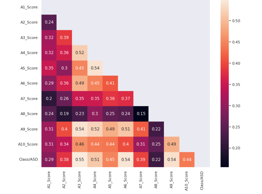
To understand the correlation of A1 to A10 feature scores with the class variable we plot the below heatmap.
correlation_columns = []
for col in score_columns:
    correlation_columns.append(col)
correlation_columns.append("Class/ASD")
correlation = train[correlation_columns].corr()
mask = np.<a onclick="parent.postMessage({'referent':'.numpy.triu'}, '*')">triu(np.<a onclick="parent.postMessage({'referent':'.numpy.ones_like'}, '*')">ones_like(correlation, dtype=np.<a onclick="parent.postMessage({'referent':'.numpy.bool'}, '*')">bool))
plt.<a onclick="parent.postMessage({'referent':'.matplotlib.pyplot.figure'}, '*')">figure(figsize=(11, 9))
sns.<a onclick="parent.postMessage({'referent':'.seaborn.heatmap'}, '*')">heatmap(correlation,annot=True,mask=mask)
Source: Author
A3, A6, A9, A4, A5, and A10 have a correlation higher than 0.4
Let’s find out how age correlates with the target
correlation = train[["age","result","Class/ASD"]].corr()
mask = np.<a onclick="parent.postMessage({'referent':'.numpy.triu'}, '*')">triu(np.<a onclick="parent.postMessage({'referent':'.numpy.ones_like'}, '*')">ones_like(correlation, dtype=np.<a onclick="parent.postMessage({'referent':'.numpy.bool'}, '*')">bool))
plt.<a onclick="parent.postMessage({'referent':'.matplotlib.pyplot.figure'}, '*')">figure(figsize=(11, 9))
sns.<a onclick="parent.postMessage({'referent':'.seaborn.heatmap'}, '*')">heatmap(correlation,annot=True,mask=mask)
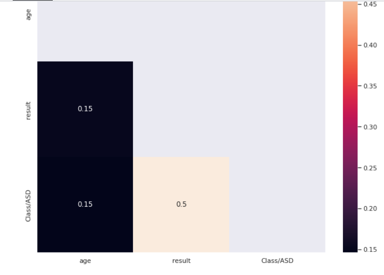
Age does not seem to have a very high correlation value with the target
For understanding the relationship between gender and target we plot the below.
sns.<a onclick="parent.postMessage({'referent':'.seaborn.boxplot'}, '*')">boxplot(data=train,x='gender',y='Class/ASD')
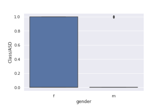
from sklearn.preprocessing import LabelEncoder
le = LabelEncoder()
transformed_gender = le.fit_transform(train["gender"])
train["transformed_gender"] = transformed_gender
corre = train[["transformed_gender","Class/ASD"]].corr()
sns.<a onclick="parent.postMessage({'referent':'.seaborn.heatmap'}, '*')">heatmap(corre,annot=True)
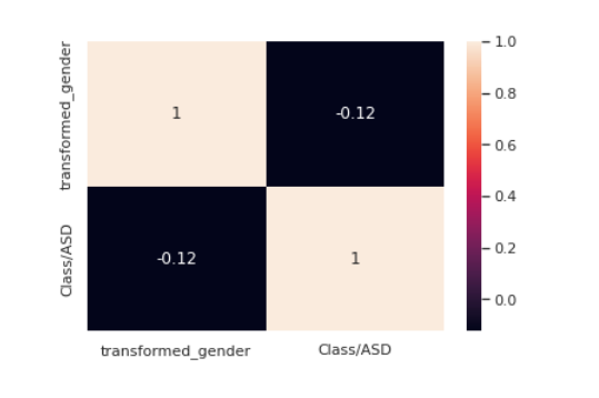
The correlation between gender and target seems to be weak.
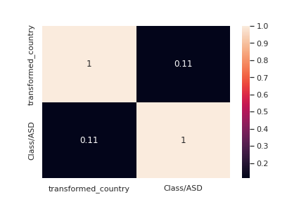
Can the country where the patient resides have an effect? Let’s find out.
plt.<a onclick="parent.postMessage({'referent':'.matplotlib.pyplot.figure'}, '*')">figure(figsize=(20, 15))
top_5  = ["United States", "United Arab Emirates", "New Zealand", "India" , "United Kingdom"]
train_subset = train.loc[train["contry_of_res"].isin(top_5)]
sns.<a onclick="parent.postMessage({'referent':'.seaborn.boxplot'}, '*')">boxplot(data=train_subset,x='contry_of_res',y='Class/ASD')
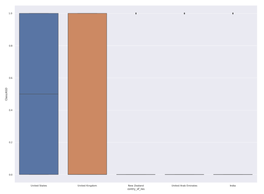
le = LabelEncoder()
transformed_country = le.fit_transform(train["contry_of_res"])
train["transformed_country"] = transformed_country
corre = train[["transformed_country","Class/ASD"]].corr()
sns.<a onclick="parent.postMessage({'referent':'.seaborn.heatmap'}, '*')">heatmap(corre,annot=True)
Let us now see if ethnicity correlates with our target
chart = sns.<a onclick="parent.postMessage({'referent':'.seaborn.boxplot'}, '*')">boxplot(data=train,x='ethnicity',y='Class/ASD')
chart.set_xticklabels(chart.get_xticklabels(), rotation=45)
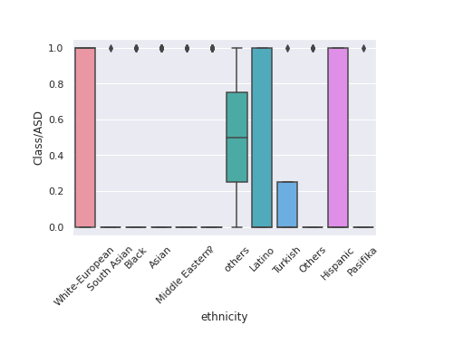
It seems we have two values others and Others in the ethnicity feature which have the same meaning. Let’s clean it out
train['ethnicity'] = train['ethnicity'].replace('others','Others')
le = LabelEncoder()
transformed_ethnicity = le.fit_transform(train["ethnicity"])
train["transformed_ethnicity"] = transformed_ethnicity
corre = train[["transformed_ethnicity","Class/ASD"]].corr()
sns.<a onclick="parent.postMessage({'referent':'.seaborn.heatmap'}, '*')">heatmap(corre,annot=True)
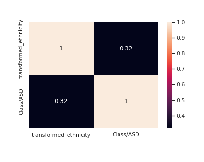
Ethnicity seems to have a decent correlation with the target
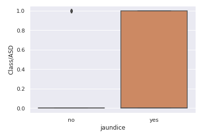
Understanding the relationship between jaundice and the target
chart = sns.<a onclick="parent.postMessage({'referent':'.seaborn.boxplot'}, '*')">boxplot(data=train,x='jaundice',y='Class/ASD')
le = LabelEncoder()
transformed_jaundice = le.fit_transform(train["jaundice"])
train["transformed_jaundice"] = transformed_jaundice
corre = train[["transformed_jaundice","Class/ASD"]].corr()
sns.<a onclick="parent.postMessage({'referent':'.seaborn.heatmap'}, '*')">heatmap(corre,annot=True)
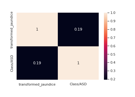
Jaundice seems to have a decent correlation with the target
Correlation of autism feature with the target variable
le = LabelEncoder()
transformed_austim = le.fit_transform(train["austim"])
train["transformed_austim"] = transformed_austim
corre = train[["transformed_austim","Class/ASD"]].corr()
sns.<a onclick="parent.postMessage({'referent':'.seaborn.heatmap'}, '*')">heatmap(corre,annot=True)
transformed_austim_te = le.fit_transform(test["austim"])
test["transformed_austim"] = transformed_austim_te
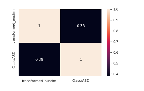
Autism seems to have a decent correlation with the target
le = LabelEncoder()
transformed_used_app_before = le.fit_transform(train["used_app_before"])
train["transformed_used_app_before"] = transformed_used_app_before
corre = train[["transformed_used_app_before","Class/ASD"]].corr()
sns.<a onclick="parent.postMessage({'referent':'.seaborn.heatmap'}, '*')">heatmap(corre,annot=True)
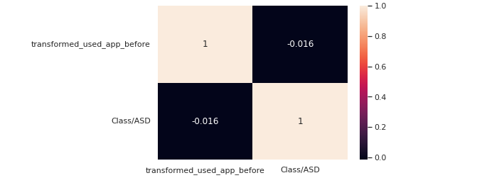
used_app_before does not have a high correlation with the target
correlation = train.corr()
mask = np.<a onclick="parent.postMessage({'referent':'.numpy.triu'}, '*')">triu(np.<a onclick="parent.postMessage({'referent':'.numpy.ones_like'}, '*')">ones_like(correlation, dtype=np.<a onclick="parent.postMessage({'referent':'.numpy.bool'}, '*')">bool))
plt.<a onclick="parent.postMessage({'referent':'.matplotlib.pyplot.figure'}, '*')">figure(figsize=(15, 15))
sns.<a onclick="parent.postMessage({'referent':'.seaborn.heatmap'}, '*')">heatmap(correlation,annot=True,mask=mask)
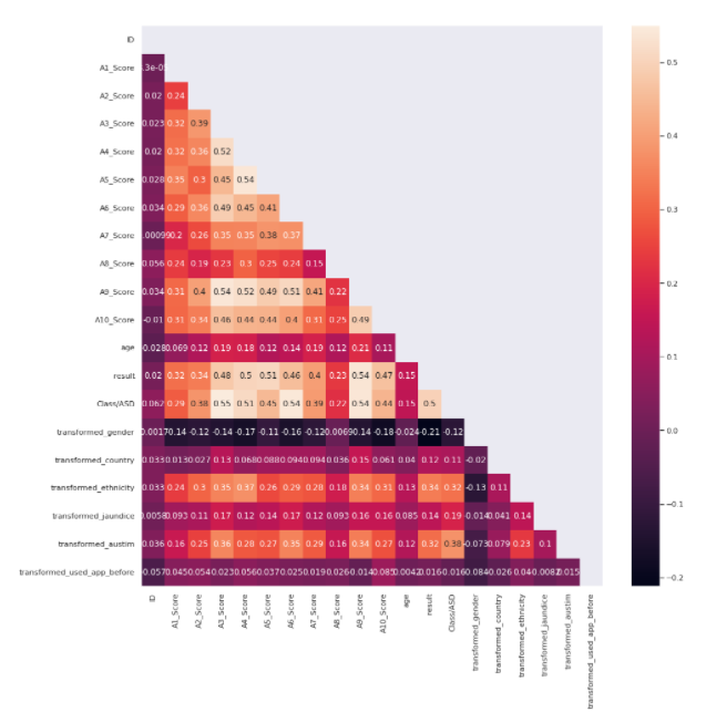
Features with the Highest Correlation to the Target
A3_Score
A2_Score
A4_Score
A5_Score
A6_Score
A7_Score
A9_Score
A10_Score
Autism
Ethnicity
Result
We would keep only these features in our data frame which would be used as input for our model.
train = train[["A3_Score","A2_Score","A4_Score","A5_Score","A6_Score","A7_Score","A9_Score","A10_Score","transformed_austim","Class/ASD","result"]]
test = test[["A3_Score","A2_Score","A4_Score","A5_Score","A6_Score","A7_Score","A9_Score","A10_Score","transformed_austim","result"]]
y = train["Class/ASD"]
train = train.drop(["Class/ASD"],axis=1)
Importing all required libraries
from sklearn.model_selection import train_test_split, StratifiedKFold, GridSearchCV
from sklearn.preprocessing import StandardScaler, OneHotEncoder, LabelEncoder
from sklearn.impute import SimpleImputer
from sklearn.pipeline import make_pipeline
from sklearn.compose import make_column_transformer
from sklearn.metrics import confusion_matrix, ConfusionMatrixDisplay, accuracy_score
from sklearn.ensemble import RandomForestClassifier

# Models
from xgboost import XGBClassifier, XGBRegressor
from catboost import CatBoostClassifier
from lightgbm import LGBMClassifier
from sklearn.linear_model import LogisticRegression
Baseline Model
I used logistic regression as my baseline model for this problem. I have used grid search CV and Stratified K Fold with 5 folds for hyper-parameter optimization.
# Define model
model=LogisticRegression(random_state=0,class_weight='balanced')

# Parameters grid
grid_model = LogisticRegression(solver='saga',
                              C=0.22,
                              penalty='l2',class_weight='balanced')

# Cross validation
kf = StratifiedKFold(n_splits=5, shuffle=True, random_state=0)

# Grid Search
#grid_model = GridSearchCV(model,param_grid,cv=kf)

# Train classifier with optimal parameters
grid_model.fit(train,y)
predictions = grid_model.predict(test)
pred_df = pd.<a onclick="parent.postMessage({'referent':'.pandas.DataFrame'}, '*')">DataFrame()
pred_df["ID"] = test_df["ID"]
pred_df["Class/ASD"] = predictions
pred_df[['ID', 'Class/ASD']].to_csv('submission.csv', index=False)
LightGBM
This gave me the highest performance on the public leaderboard with an AUC score of 0.931 and a private leaderboard score of 0.987
Conclusion
This could be a comprehensive starter for anyone who wants to try their hand out with Kaggle competitions.
What you must keep in mind before solving a data science problem.
1) Study the data religiously, understanding your data thoroughly will only help you to win a competition or for that matter get good results.
2) Start with a baseline model result.
3) Use bagging and boosting aggregation techniques if your problem involves classifying. If you have understood your data well, it would not be too difficult for you to select the correct model.
About the Author
I am an Analyst and like to interrogate data and share my findings through technical articles. You can read other articles published by me on Analytics Vidhya here. You can reach out to me here.
The media shown in this article is not owned by Analytics Vidhya and are used at the Author’s discretion.


