.png)
This article was published as a part of the Data Science Blogathon
Introduction
In this article, I am going to share my approach to solving the problem. I hope this article helps more and more people in learning new ways to approach the problem. In this article, I am going through the entire journey of getting started with this data set.
Problem Statement
In Analytics Vidya – Cross-Sell Prediction, the participants are asked to build a model to predict whether a customer would be interested in Vehicle Insurance is extremely helpful for the company because it can then accordingly plan its communication strategy to reach out to those customers and optimize its business model and revenue.
Solution
Here is the step by step solution of this competition:
Step 1. Hypothesis Testing
Before starting the data exploration to understand the relation between the independent features it is important to focus on Hypothesis Testing.
Hypothesis Testing is the first step we should take towards understanding the dataset and the business problem. The main aim of Hypothesis Testing is to give us a head-start towards understanding the problem.
I came up with the following hypothesis while thinking about the problem. These are just my thoughts and you can come up with many more of these.
1. Gender: Males are more likely to buy Vehicle Insurance.
2. Age: It is generally said that it is profitable to buy Insurance as early as possible so more likely between Customers of ages of 25-40 are likely to buy Insurance.
3. Driving_License: Customers who generally have Driving_License take Insurance.
4. Previously_Insured: Customers generally take One Vehicle insurance.
5. Vehicle_Age: The more the age of the vehicle the better.
6. Annual_Premium: Customers generally opt for Insurance where the premium is not too high.
These are just some basic 6 hypotheses I have made, but you can think further and create some of your own.
Step2. Data Exploration
In this section, we’ll try to understand the variables given in our dataset and come up with some inferences about the data.
The first step is to look at the data and try to identify the information.
| Variable | Definition |
| id | Unique ID for the customer |
| Gender | Gender of the customer |
| Age | Age of the customer |
| Driving_License | 0 : Customer does not have DL, 1 : Customer already has DL |
| Region_Code | Unique code for the region of the customer |
| Previously_Insured | 1 : Customer already has Vehicle Insurance, 0 : Customer doesn’t have Vehicle Insurance |
| Vehicle_Age | Age of the Vehicle |
| Vehicle_Damage | 1 : Customer got his/her vehicle damaged in the past. 0 : Customer didn’t get his/her vehicle damaged in the past. |
| Annual_Premium | The amount customer needs to pay as premium in the year |
| Policy_Sales_Channel | Anonymised Code for the channel of outreaching to the customer ie. Different Agents, Over Mail, Over Phone, In Person, etc. |
| Vintage | Number of Days, Customer has been associated with the company |
| Response | 1 : Customer is interested, 0 : Customer is not interested |
The training data set has 12 variables (see above) and Test has 11 (excluding Response).
Step3. Exploratory Data Analysis (EDA)
a. Let’s start by loading the required libraries and data.
import pandas as pd
import numpy as np
import matplotlib.pyplot as plt
import seaborn as sns
%matplotlib inline
test_org=pd.read_csv('test.csv')
train=train_org.copy()
test=test_org.copy()
train_org=pd.read_csv('train.csv')
b. Combine both Train and Test Data set
It is a good idea to combine both train and test data sets into one, perform Feature Engineering and then divide them later again. This saves the trouble of performing the same steps twice on test and train. Let us combine them into a data frame ‘data’ with a ‘source’ column specifying where each observation belongs.
train['source']='train'
test['source']='test'
data=pd.concat([train,test],ignore_index=True)
c. Dataset description
data.describe()
.png)
d. Find missing values in the dataset if any.
data.isnull().sum()
id                           0
Gender                       0
Age                          0
Driving_License              0
Region_Code                  0
Previously_Insured           0
Vehicle_Age                  0
Vehicle_Damage               0
Annual_Premium               0
Policy_Sales_Channel         0
Vintage                      0
Response                127037
source                       0
dtype: int64
As we can see there are no missing values in the dataset except for the Target variable (Response) that’s because we have combined our dataset and these missing values belong to the test dataset.
e. Let us plot a histogram for each numerical variable and analyze the distribution.
data.hist(figsize=(20,15),layout=(3,6))
plt.tight_layout()
plt.show()
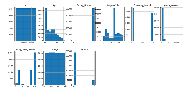
From the above plot we can see that:
– Age column is Right-Skewed.
– Response variable has an unbalanced ratio in labels. So we will apply some techniques later in the model building stage.
– Diriving_license column has an unbalanced ratio between the labels.
As we know that Diriving_license column has an unbalanced ratio between the labels so we can delete this column.
data.drop('Driving_License',axis=1,inplace=True)
f. Numerical and Categorical variables analysis
sns.barplot(x='Gender',y='Response',data=data)
plt.title('Gender')
plt.show()
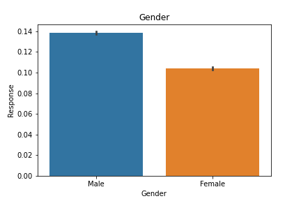
As we can see that Males are more likely to buy Vehicle Insurance which proves our Hypothesis also.
sns.barplot(x='Vehicle_Age',y='Response',data=data)
plt.show()
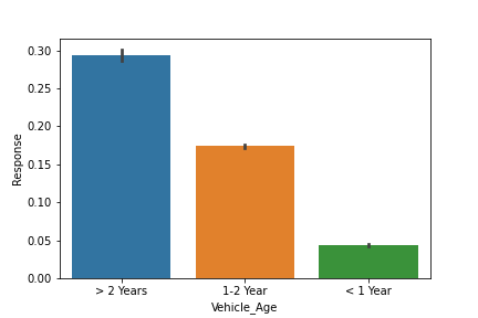
From the above figure, it is clear that the more the age of the vehicle the better as it makes the vehicle insurance cheaper
To know more about the correlation between Vehicle insurance and Vehicle age refer to this link
Feel free to dig deeper and find more insights from the dataset. We will move to the next section that is Data Cleaning.
Step4. Data Cleaning
This step typically involves imputing missing values, treating outliers, and performing Encoding. We can perform encoding either by manually using the map() or by using LabelEncoder().
gender_map={'Male':0,'Female':1}
data['Gender']=data['Gender'].map(gender_map)
vehicle_age_map={'1-2 Year':0,'< 1 Year':1,'> 2 Years':2}
data['Vehicle_Age']=data['Vehicle_Age'].map(vehicle_age_map)
Vehicle_Damage_map={'Yes':0,'No':1}
data['Vehicle_Damage']=data['Vehicle_Damage'].map(Vehicle_Damage_map)
Now we will move to the next section Feature Engineering.
Step5. Feature Engineering
In addition to existing independent variables, we will create new variables to improve the prediction power of the model.
In this section, we will try the Discretisation of continuous variables using Decision Tree.
Discretization is a process of converting the continuous variable into a discrete variable with the help of bins. It also helps in removing Outliers as after converting into bins the Outliers fall in the interval
In this section, we will convert the continuous variable (‘Age’, ‘Annual_Premium’) into discrete variables
Steps to Follow:
1. Spit the data into train_test and fit the Decision Tree (depth=1,2,3,4) using the X= continuous variable ; y=Target
2. The continuous variable is then replaced by the predicted_probability.
X=data.loc[data['source']=='train',['Age','Annual_Premium','Response']]
y=data.loc[data['source']=='train',['Response']]
x_train,x_test,y_train,y_test = train_test_split(X,y,test_size = 0.30 ,random_state = 2)
## Fit the tree
dtree=DecisionTreeClassifier(max_depth=2)
dtree.fit(x_train.Age.to_frame(),y_train)
## Calculate the probability
x_train['Age_tree']=dtree.predict_proba(x_train.Age.to_frame())[:,1]
x_train.groupby('Age_tree')['Response'].mean().plot()
plt.title('Monotonic Relationship with the Target.')
plt.show()
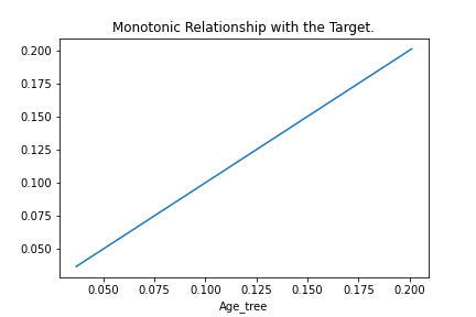
We can see that our new variable is a good predictor of the Target variable.
Further, we can use the Predicted_probability to create the Bins.
age_limit=pd.DataFrame({'Min_Age':x_train.groupby('Age_tree')['Age'].min(),'Max_Age':x_train.groupby('Age_tree')['Age'].max()})
.png)
Let’s visualize the Decision Tree graph
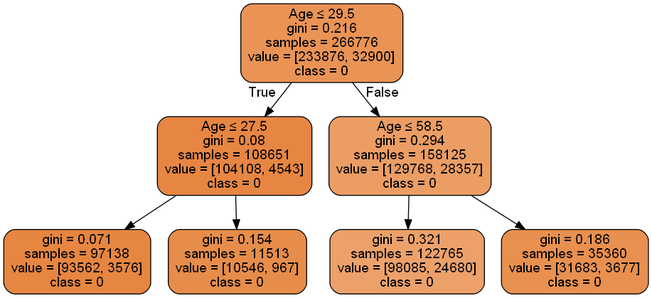
Now we can now convert the Age column using the above intervals.
data.loc[(data['Age']>=20) & (data['Age']<27),'Age_label']='Teenagers'
data.loc[(data['Age']>=27) & (data['Age']<29),'Age_label']='Young'
data.loc[(data['Age']>=29) & (data['Age']<58),'Age_label']='Middle Age'
data.loc[(data['Age']>=58) & (data['Age']<=85),'Age_label']='Old Age'
data.loc[(data['Age']>=20) & (data['Age']<27),'Age']=0 ## Just starting out
data.loc[(data['Age']>=27) & (data['Age']<29),'Age']=1 ## Young Ppl
data.loc[(data['Age']>=29) & (data['Age']<58),'Age']=2 ## Mid-Age Ppl
data.loc[(data['Age']>=58) & (data['Age']<=85),'Age']=3 ## Old Age
Let us plot our new variable and gain some insight.
sns.barplot(data['Age_label'],data['Annual_Premium'])
plt.title('Annual_Premium according to Age')
plt.show()
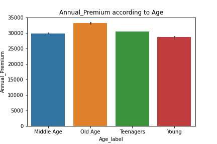
From the above plot, we can see that Annual_Premium is directly dependent on the Age of the Customer. The higher the Age higher the Annual_Premium.
Annual_Premium: Using similar methods, we have created bins for Annual_Premium.
Step6. Exporting Data
The final step is to convert data back into train and test data sets. It’s generally a good idea to export both of these as modified data sets. This can be achieved using the following code:
data=pd.get_dummies(data,columns=['Vehicle_Age','Age','Annual_Premium'],drop_first=True)
train=data.loc[data['source']=='train']
test=data.loc[data['source']=='test']
train.drop(['source','id','Age_label','Annual_Premium_label'],axis=1,inplace=True)
test.drop(['source','id','Response','Age_label','Annual_Premium_label'],axis=1,inplace=True)
With this, we come to the end of this section. If you want all the codes for exploration and feature engineering in an iPython notebook format, you can download the same from my GitHub repository.
Step7. Model Building
We will be using the ROC-AUC score as our Evaluation Metric for this competition.
You can read more about ROC-ACU from this article
a. Loading the Libraries
from sklearn.model_selection import train_test_split,cross_val_score,KFold
from sklearn.metrics import roc_auc_score
from sklearn.metrics import roc_curve
from sklearn.preprocessing import StandardScaler
from sklearn.linear_model import LogisticRegression
from sklearn.tree import DecisionTreeClassifier
from sklearn.ensemble import RandomForestClassifier
from sklearn.neighbors import KNeighborsClassifier
from xgboost import XGBClassifier
b. Train test split
X=train.drop(['Response'],axis=1)
y=train['Response'].astype('int')
x_train,x_test,y_train,y_test = train_test_split(X,y,test_size = 0.30 ,random_state = 5)
c. Handling an Unbalanced Dataset
We have earlier seen that the Response variable has an unbalanced ratio in labels. So we will apply some techniques to balance the ratio so that.
You can read more about how to handle an Unbalanced Dataset from this article
from imblearn.over_sampling import SMOTE
smote = SMOTE()
X_balanced, y_balanced = smote.fit_resample(X, y)
X_train_balanced,X_test_balanced,y_train_balanced,y_test_balanced=train_test_split(X_balanced,y_balanced,test_size=0.3,random_state=5)
d. We will be using Cross-Validation to find the model which has the best accuracy.
models=[]
models.append(('LogisticRegression',LogisticRegression(solver="liblinear", random_state=5)))
models.append(('DecisionTree',DecisionTreeClassifier(random_state=5)))
models.append(('RandomForest',RandomForestClassifier(random_state=5)))
models.append(('knn',KNeighborsClassifier()))
results=[]
names=[]
for name,model in models:
    kf=KFold(n_splits=5,shuffle=True,random_state=5)
    cv_score=cross_val_score(model,X_balanced,y_balanced,cv=kf,scoring='roc_auc',verbose=1)
    results.append(cv_score)
    names.append(name)
    msg = "%s: %f (%f)" % (name, cv_score.mean(), cv_score.std())
    print(msg)
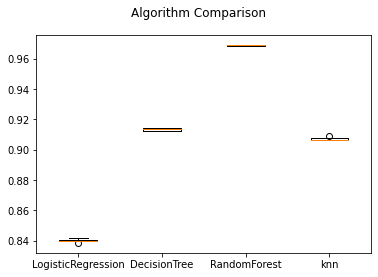
Now let’s plot the ROC-AUC curve for all the models.
for name,model in models:
#     model = m['model'] # select the model
    model.fit(x_train, y_train) # train the model
    y_pred=model.predict(x_test) # predict the test data
# Compute False postive rate, and True positive rate
    fpr, tpr, thresholds = roc_curve(y_test, model.predict_proba(x_test)[:,1])
# Calculate Area under the curve to display on the plot
    auc =roc_auc_score(y_test,model.predict(x_test))
# Now, plot the computed values
    plt.plot(fpr, tpr, label='%s ROC (area = %0.2f)' % (name, auc))
# Custom settings for the plot
plt.plot([0, 1], [0, 1],'r--')
plt.xlim([0.0, 1.0])
plt.ylim([0.0, 1.05])
plt.xlabel('1-Specificity(False Positive Rate)')
plt.ylabel('Sensitivity(True Positive Rate)')
plt.title('Receiver Operating Characteristic')
plt.legend(loc="lower right")
plt.show()   # Display
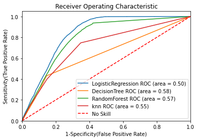
We can see that Random Forest has the highest ROC-AUC score of=0.88.
We shall further try the Ensembled methods to increase our accuracy.
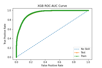
xgb=XGBClassifier(random_state=5,max_depth=5)
xgb.fit(X_train_balanced,y_train_balanced)
With XGB Classifier we got ROC-AUC score of 0.86.
Step8. Final Submission
We will be using XGB Classifier for final predictions.
predsTest = xgb.predict(test)
submission = pd.DataFrame({  "id": test_org['id'], "Response":predsTest })
submission.to_csv('XGB_submission.csv', index=False)
With this, we come to the end of this section. If you want all the codes for model building in an iPython notebook format, you can download the same from my GitHub repository
End Notes
In this article, we have looked at a structured approach to problem-solving. I would recommend you generate more hypotheses to dive deep into the dataset, which can further help us create more meaningful features. You can improve your performance by applying advanced techniques and understand your data trend better.
You
can find the complete solution here: GitHub repository
Hope you liked this article and I hope you found it very useful in achieving what you what.
You can refer to my other article here
Dishaa Agarwal I am a data science enthusiast having knowledge in Exploratory Data Analysis, Feature Engineering, worked with multiple Machine Learning algorithms and I am currently learning Deep Learning. I always try to create content in such a way that people can easily understand the concept behind the topic.
The media shown in this article are not owned by Analytics Vidhya and are used at the Author’s discretion.


