Introduction
The Hough Transform is a pivotal algorithm in computer vision and image processing, enabling the detection of geometrical shapes such as lines, circles, and ellipses within images. By transforming image space into parameter space, the Hough Transform leverages a voting mechanism to identify shapes through local maxima in an accumulator array. Typically, this method detect lines and edges, utilizing parameters like rho and theta to represent straight lines in polar coordinates. This algorithm is essential in various applications, from edge detection and feature extraction to more complex tasks like circle detection and generalized shape identification. Implemented in languages like Python, often using libraries like OpenCV, the hough transform line detection remains a robust tool for analyzing and interpreting visual data despite its computational intensity and parameter sensitivity.
This article will provide you with in-depth knowledge about the Hough transform. It will give you a basic introduction to the Hough transform, how exactly it works, and the math behind it. It also enlists the merits and demerits of Hough Transform algorithm and its various applications.
Learning Outcomes:
- Explain the foundational concepts of the Hough Transform, including its purpose in detecting geometrical shapes within images, and its historical development.
- Gain an understanding of the mathematical principles underlying the Hough Transform, such as the transformation of image space to parameter space.
- Implement the Hough Transform line detection algorithm in a programming language such as Python using libraries like OpenCV.
- Explore various real-world applications of the Hough Transform algorithm, such as in-lane and traffic sign recognition, medical imaging, industrial inspection, and object tracking.
This article was published as a part of the Data Science Blogathon.
Table of contents
History
It was first developed for the automated examination of bubble chamber pictures (Hough, 1959). In 1962, the Hough transform was patented as U.S. Patent 3069654 and assigned by the Atomic Energy Commission to the United States as a “Method and Means for Recognizing Complex Patterns.” Because the slope might go to infinity, this invention employs a slope-intercept parameterization for straight lines, which results in infinite transform space.
Duda, R. O., and P. E. Hart, “Use of the HT to Detect Lines and Curves in Pictures,” Comm. ACM, Vol. 15, pp. 11–15 (January 1972), although it had been standard for the Radon transformation since the 1930s. In Frank O’Gorman and MB Clowes: Finding Picture Edges through Collinearity of Feature Points, O’Gorman and Clowes discuss their version. IEEE Transactions on Computers, vol. 25, no. 4, pp. 449-456. (1976) Hart, P. E., “How the HT was invented,” IEEE Signal Processing Magazine, Vol 26, Issue 6, pages 18 – 22 (November 2009) tells the tale of how the contemporary form of the Hough transform was invented.
What is Hough Transform?
Hough Transform is a computer vision technique that detects shapes like lines and circles in an image. It converts these shapes into mathematical representations in parameter space, making it easier to identify them even if they’re broken or obscured. This method is valuable for image analysis, pattern recognition, and object detection.
The Hough Transform algorithm line detection is a feature extraction method in image analysis, computer vision, and digital image processing. It uses a voting mechanism to identify bad examples of objects inside a given class of forms. This voting mechanism is carried out in parameter space. First, the HT algorithm produces object candidates as local maxima in an accumulator space.
The traditional HT was concerned with detecting lines in an image, but it was subsequently expanded to identifying locations of arbitrary shapes, most often circles or ellipses. Richard Duda and Peter Hart devised the HT as we know it today in 1972, calling it a “generalized HT” after Paul Hough’s related 1962 patent. Dana H. Ballard popularized the transformation in the computer vision field with his 1981 journal paper “Generalizing the HT to Identify Arbitrary Forms.”
Why is it Needed?
In many circumstances, a pre-processing stage can use an edge detector to obtain picture points or pixels on the required curve in the image space. However, there may be missing points or pixels on the required curves due to flaws in either the image data or the edge detector and spatial variations between the ideal line/circle/ellipse and the noisy edge points acquired by the edge detector. As a result, grouping the extracted edge characteristics into an appropriate collection of lines, circles, or ellipses is frequently difficult.

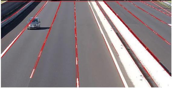
1. Original image of Lane
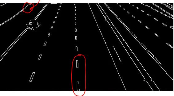
Figure 2: Image after applying edge detection technique. Red circles show that the line is breaking there.
How Does the Hough Transform Work?
The Hough approach is effective for computing a global description of a feature(s) from (potentially noisy) where the number of solution classes does not need to be provided. For example, the Hough approach for line identification motivates the assumption that each input measurement reflects its contribution to a globally consistent solution (e.g., the physical line that gave rise to that image point).
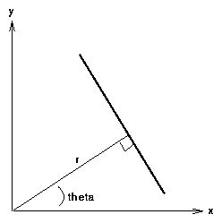
A line can be described analytically in various ways. One of the line equations uses the parametric or normal notion: xcosθ+ysinθ=r. where r is the length of a normal from the origin to this line and θ is the orientation, as given in Figure 5.
The known variables (i.e., x i,y i ) in the image are constants in the parametric line equation, whereas r and are the unknown variables we seek. Points in cartesian image space correspond to curves (i.e., sinusoids) in the polar Hough parameter space if we plot the potential (r, θ) values specified by each. The Hough Transform algorithm for straight lines is this point-to-curve transformation. Collinear spots in the cartesian image space become obvious when examined in the Hough parameter space because they provide curves that overlap at a single (r, θ) point.
A and b are the circle’s center coordinates, and r is the radius. The algorithm’s computing complexity increases because we now have three coordinates in the parameter space and a 3-D accumulator. (In general, the number of parameters increases the calculation and the size of the accumulator array polynomially.) As a result, the fundamental Hough approach described here only applies to straight lines.
Algorithm
- Determine the range of ρ and θ. Typically, the range of θ is [0, 180] degrees and ρ is [-d, d], where d is the diagonal length of the edge. Therefore, it’s crucial to quantify the range of ρ and θ, which means there should only be a finite number of potential values.
- Create a 2D array called the accumulator with the dimensions (num rhos, num thetas) to represent the Hough Space and set all its values to zero.
- Use the original image for edge detection (ED). You can use whatever ED technique you like.
- Check each pixel on the edge picture to see if it is an edge pixel. If the pixel is on edge, loop over all possible values of θ, compute the corresponding ρ, locate the θ and ρ index in the accumulator, and then increase the accumulator base on those index pairs.
- Iterate over the accumulator’s values. Retrieve the ρ and θ index and get the value of ρ and θ from the index pair. If the value exceeds a specified threshold, we can then transform the index pair back to the form of y = ax + b.
Sum of Hough Transform
Problem: Given set of points, use Hough transform to join these points. A(1,4), B(2,3) ,C(3,1) ,D(4,1) ,E(5,0)
Solution:
Lets think about equation of line that is y=ax+b.
Now, if we rewrite the same line equation by keeping b in LHS, then we get
b=-ax+y. So if we write the same equation for point A(1,4), then consider x=1 and y=4 so that we will get
b=-a+4. The following table shows all the equations for a given point
| Point | X and y values | Substituting the value in b=-ax+y |
| A(1,4) | x=1 ; y=4 | b= -a+4 |
| B(2,3) | x=2 ; y=3 | b= -2a+3 |
| C(3,1) | x=3 ; y=1 | b= -3a+1 |
| D(4,1) | x=4 ; y=1 | b= -4a+1 |
| E(5,0) | x=5 ; y=0 | b= -5a+0 |
Now take x-0 and find corresponding y value for above given five equations
| Point | equations | Now a=0 | New point (a,b) | Now a=1 | New point (a,b) |
| A(1,4) | b= -a+4 | b= -(0)+4 =4 | (0,4) | b= -(1)+4 =3 | (1,3) |
| B(2,3) | b= -2a+3 | b= -2(0)+3=3 | (0,3) | b= -2(1)+3=1 | (1,1) |
| C(3,1) | b= -3a+1 | b= -3(0)+1=1 | (0,1) | b= -3(1)+1=-2 | (1,-2) |
| D(4,1) | b= -4a+1 | b= -4(0)+1=1 | (0,1) | b= -4(1)+1=3 | (1,-3) |
| E(5,0) | b= -5a+0 | b= -5(0)+0=0 | (0,0) | b= -5(1)+0=-5 | (1,-5) |
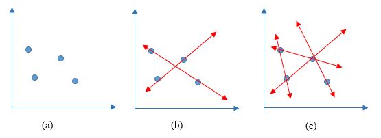
Let us plot the new point on the graph as given below in figure 6.
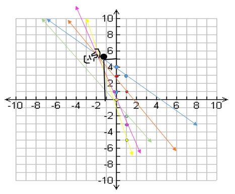
We can see that almost all line crosses each other at a point (-1,5). So here now a=-1 and b =5.
Now let’s put these values in the y=ax+b equation so we get y=-1x+5 so y=-x+5 is the line equation that will link all the edges.
Advantages of Hough Transform
- Robustness: It can detect shapes in images even if they are partially obscured, degraded, or noisy.
- Simplicity: Conceptually straightforward, making it relatively easy to implement and understand.
- Versatility: Can be adapted to detect various geometric shapes, not just lines but also circles and ellipses.
- Global Detection: Able to identify lines and shapes across the entire image rather than just in localized regions.
Disadvantages of Hough Transform
- Computationally Intensive: This can be slow and requires significant computational resources, especially for large images or complex shapes.
- Parameter Sensitivity: Requires careful selection of parameters (e.g., resolution of the parameter space) to balance accuracy and performance.
- Noise Sensitivity: This may produce false positives if the image has a lot of noise or clutter.
- Discrete Nature: Quantizing the parameter space can lead to a loss of precision in detecting shapes.
Application of the Hough Transform
The HT has been widely employed in numerous applications because of the benefits, such as noise immunity. 3D applications, object and form detection, lane and traffic sign recognition, industrial and medical applications, pipe and cable inspection, and underwater tracking are just a few examples [6]. Below are some examples of these applications. Proposes the hierarchical additive Hough transform (HAHT) for detecting lane lines. The HAHT that is recommended accumulates the votes at various hierarchical levels. Line segmentation into multiple blocks also minimizes the computational load. [7] proposes a lane detection strategy in which the HT is merged with the joint photographic experts’ group (JPEG) compression. However, only simulations are used to test the method.
Biometric and Man-machine Interaction
A generalized hand detection model with articulated degrees of freedom is shown in 6. It makes use of geometric feature correspondences between points and lines. The PHT recognizes the lines. Following that, they are matched with a model. The GHT can identify Turkish finger-spelling. To produce interest zones, the scale-invariant features transform is applied (SIFT). The superfluous interest zones are eliminated using skin color reduction. It also suggests using hand gestures and tracking to create a real-time human-robot interaction system. The linked component labeling (CCL) and the Hough transform are integrated into this procedure. Sensing the skin tone can extract the hand’s center, orientations, and fingertip positions of all outstretched fingers.
3D Applications
It proposes a detector for 3D lines, boxes, and blocks. This approach decreases the computing cost by using 2D Hough space for parallel line detection. In addition, 3D HT is used to extract planar faces from point clouds that are unevenly dispersed.
Object Recognition
It describes a method for detecting objects utilizing the GHT and color similarity between homogeneous portions of the item. It takes as input already segmented areas of homogenous hue. According to this research, it resists changes in light, occlusion, and distortion of the segmentation output. It can distinguish items that have been rotated, scaled, and even moved around in a complicated environment.
Object Tracking
It uses a blend of uniform and Gaussian Hough transforms to conduct shape-based tracking. While the camera moves, this method can find and follow objects even against difficult backdrops like a dense forest.
Underwater Application
It offers a technique for detecting geometrical forms in underwater robot images. Unlike the traditional Generalized Hough Transform (GHT), it transforms the recognition problem into a bounded error estimation problem. An autonomous underwater vehicle (AUV) creates a system for visually directed operations underwater. The Hough Transform identifies underwater pipelines, and their orientations are determined using binary morphology.
Industrial and Commercial Application
Various industrial and commercial uses utilize the Hough Transform (HT) and its various versions. For instance, in an uncrewed aerial vehicle (UAV) surveillance and inspection system, a knowledge-based power line identification approach is proposed. Before applying the Line Hough Transform (LHT), researchers construct a pulse-coupled neural network (PCNN) filter to eliminate background noise from picture frames. They then refine the findings using knowledge-based line clustering.
Medical Application
It uses a warped frequency transform (WFT) to adjust for the dispersive behavior of ultrasonic guided waves, followed by a Wigner-Ville time-frequency analysis and the HT to increase fault localization accuracy. The system automatically recognizes the locations and boundaries of vertebrae. It utilizes the Hough Transform in conjunction with the Genetic Algorithm to determine the migrating vertebrae.
Unconventional Application
This section shows unexpected usage to demonstrate the HT’s adaptability and ever-expanding nature. It proposes a data mining technique for locating arbitrarily oriented subspace clusters. This is achieved by mapping the data space to the parameter space, defining the collection of arbitrarily oriented subspaces that may be created. The clustering method works by locating clusters that may hold many database objects. Even if subspace clusters of differing dimensions are sparse or crossed by other clusters in a noisy environment, the method can discover them.
Implementation Using the Hough Transform
Code for Line detection using hough transform
Python Code:
import numpy as np
import cv2
# import opencv-python
# Read image
img = cv2.imread('lane_hough.jpg',cv2.IMREAD_COLOR) # road.png is the filename
# Convert the image to grayscale
gray = cv2.cvtColor(img, cv2.COLOR_BGR2GRAY)
# Find the edges in the image using canny detector
edges = cv2.Canny(gray, 50, 200)
# Detect points that form a line
lines = cv2.HoughLinesP(edges, 1, np.pi/180, 68, minLineLength=15, maxLineGap=250)
#lines = cv2.HoughLinesP(edges, 1, np.pi/180, minLineLength=10, maxLineGap=250)
# Draw lines on the image
for line in lines:
x1, y1, x2, y2 = line[0]
cv2.line(img, (x1, y1), (x2, y2), (255, 0, 0), 3)
# Show result
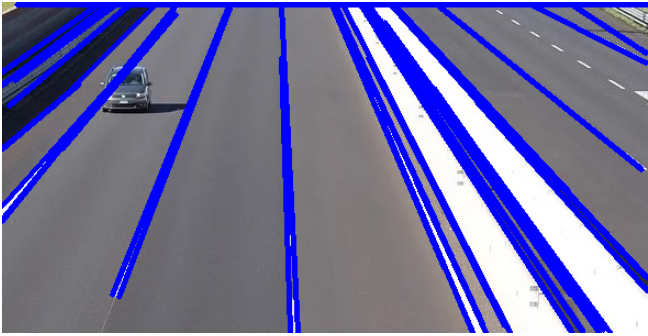
print("Line Detection using Hough Transform")
cv2.imshow('lanes',img)
cv2.waitKey(0)
cv2.destroyAllWindows()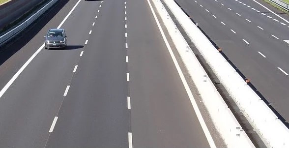
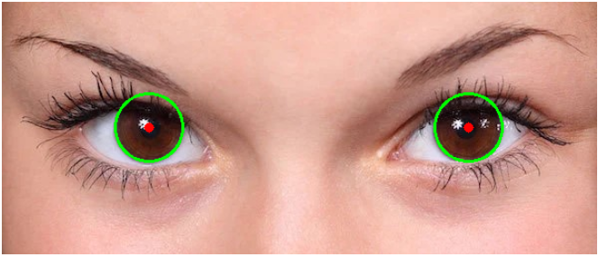
Circle Detection Using Hough Transform
# Read image as gray-scale
 img = cv2.imread('/content/drive/MyDrive/Colab Notebooks/circle_hough.jpg', cv2.IMREAD_COLOR)
 # Convert to gray-scale
 print("Original Image")
 cv2_imshow(img)
 gray = cv2.cvtColor(img, cv2.COLOR_BGR2GRAY)
 # Blur the image to reduce noise
 img_blur = cv2.medianBlur(gray, 5)
 # Apply hough transform on the image
 circles = cv2.HoughCircles(img_blur, cv2.HOUGH_GRADIENT, 1, 40, param1=100, param2=30, minRadius=1, maxRadius=40)
 # Draw detected circles
 if circles is not None:
     circles = np.uint16(np.around(circles))
     for i in circles[0, :]:
         # Draw outer circle
         cv2.circle(img, (i[0], i[1]), i[2], (0, 255, 0), 2)
         # Draw inner circle
         cv2.circle(img, (i[0], i[1]), 2, (0, 0, 255), 5)
 # Show result
 print("Circle Detection using Hough Transform")
 cv2_imshow(img)
Output
Conclusion
The Hough transform is a robust image processing technique for detecting geometric shapes in noisy and occluded images. By transforming points from image space to parameter space, it identifies local maxima in an accumulator array to detect shapes like lines, circles, and ellipses. Despite computational intensity and parameter sensitivity, its global detection capabilities make it invaluable in applications such as lane recognition, medical imaging, and industrial inspection. Parallel computing advancements promise to enhance its efficiency for real-time use, solidifying its role as a fundamental computer vision tool.
Key Takeaways:
- Hough Transform detects shapes by transforming points to parameter space
- Voting mechanism makes it robust to noise and missing data
- Wide applications: lane recognition, medical imaging, industrial inspection, etc.
- Fundamental tool despite computational intensity; efficiency improving with parallel computing
Frequently Asked Questions
Q1. What is the Hough transform used for?
A. The Hough transform is a feature extraction technique used in image analysis, computer vision, and digital image processing. It particularly excels at detecting simple shapes like lines, circles, and ellipses in images, even if these shapes are partially obscured or distorted.
Q2. What is the equation for the Hough transform?
A. The equation for the Hough transform, specifically for detecting lines, maps points from the Cartesian coordinate system (x,y) to the polar coordinate system (ρ,θ). The equation is:
ρ=xcos(θ)+ysin(θ)
Q3. How does Hough circle transform work?
A. The Hough Circle Transform is an extension of the Hough Transform used to detect circles. Each point in the image votes for all possible circles that could pass through that point. The process involves:
1- Mapping each edge point to a circular parameter space.
2- Accumulating votes in an accumulator matrix for possible circle centers and radii.
3- Identifying local maxima in the accumulator matrix, which correspond to the most likely circle parameters (center and radius).
Q4. What is the Hough line method?
A. The Hough Line Method is a specific application of the Hough Transform for detecting lines in an image. Steps involved:
a) Convert the image to an edge-detected version (using methods like Canny edge detection).
b) For each edge point, calculate all possible lines that could pass through that point and vote for them in the Hough space (ρ, θ).
c) Identify the peaks in the Hough space, which represent the most probable lines in the image.
This method is robust to noise and can detect lines even when parts of them are missing.
The media shown in this article is not owned by Analytics Vidhya and is used at the Author’s discretion.
Dr. Dulari Bhatt is Master Trainer at Edunet Foundation. She is having 12 years of experience in academia. Her main research interests are in the field of Big Data Analytics, Computer Vision, Machine Learning, and Deep Learning. She has authored 3 technical books and published several research papers in reputed international journals. She is an active writer in Analytics Vidhya and OSFY magazine. She has received a gold category award from GTU for spreading IPR awareness. Several times winner of Data Science Blogathons..


