Introduction to Saliency Map in an Image with TensorFlow 2.x API

Introduction

In the field of computer vision, a saliency map of an image in the region on which a human’s sight focuses initially. The main goal of a saliency map is to highlight the importance of a particular pixel to the human’s visual perception. For example, in the image below, the flower and human hand are the first things a person notices, so they must be emphasized on the saliency map. One more thing to be seen is that the saliency maps created by the artificial neural network are not always the same as those produced by biological or natural vision.

This article was published as a part of the Data Science Blogathon.

What is a Saliency Map?

 The saliency map is a key theme in deep learning and computer vision. During the training of a deep convolutional neural network, it becomes essential to know the feature map of every layer. The feature maps of CNN tell us the learning characteristics of the model. Suppose we want to focus on a particular part of an image than what concept will help us. Yes, it is a saliency map. It mainly focuses on specific pixels of images while ignoring others.

Saliency Map

The saliency map of an image represents the most prominent and focused pixel of an image. Sometimes, the brighter pixels of an image tell us about the salient of the pixels. This means the brightness of the pixel is directly proportional to the saliency of an image.

Suppose we want to give attention to a particular part of an image, like wanting to focus on the image of a bird rather than the other parts like the sky, nest etc. Then by computing the saliency map, we will achieve this. It will crucially assist in reducing the computational cost. It is usually a grayscale image but can be converted into another format of a coloured image depending upon our visual comfortability. Saliency maps are also termed “heat maps” since the hotness/brightness of the image has an impactful effect on identifying the class of the object. The saliency map aims to determine the areas in the fovea that are salient or observable at every place and to influence the decision of attentive regions based on the spatial pattern of saliency. It is employed in a variety of Visual Attention models. The “ITTI and Koch” Computational Framework of Visual Attention is built on the notion of a saliency map.

How to Compute Saliency Map with Tensorflow?

The saliency map can be calculated by taking the derivatives of the class probability P_k with respect to the input image X.

saliency_map = dp_k/dX

Hang on a minute! That seems quite familiar! Yes, it’s the same backpropagation which we use for training the model. We only need to take one more step: the gradient does not stop at the first layer of our network. Rather, we must return it to the input image X.

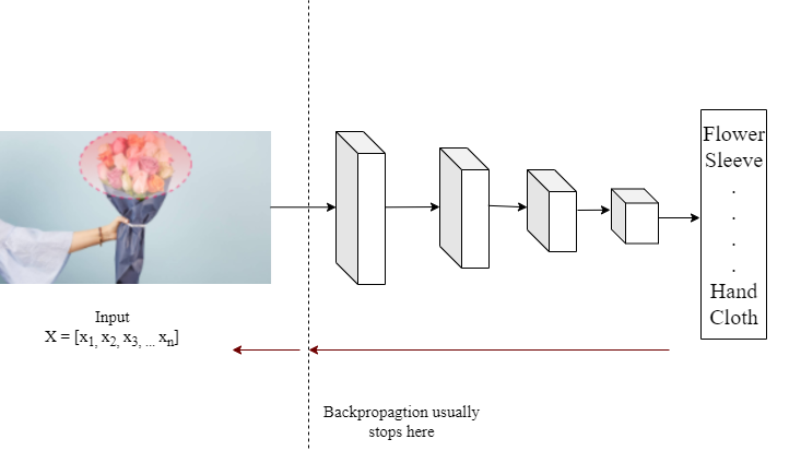
As a result, saliency maps provide a suitable characterization for each input pixel in accordance with a specific class prediction P_i. Pixels that are significant for flower prediction should cluster around flower pixels. Otherwise, something really strange is going on with the trained model.

The advantage of saliency maps is that, since they depend exclusively on gradient computations, many commonly used deep learning models can provide us with saliency maps for free. We don’t need to modify the network architectures at all; we simply need to tweak the gradient calculations slightly.

Different Types of the Saliency Map

1. Static Saliency: It focuses on every static pixel of the image to calculate the important area of interest for saliency map analysis.

2. Motion Saliency: It focuses on the dynamic features of video data. The saliency map in a video is computed by calculating the optical flow of a video. The moving entities/objects are considered salient objects.

Code

We will perform step-by-step investigations of the ResNet50 architecture, which has been pre-trained on ImageNet. But you can take other pretrained deep learning models or bring your own trained model. We will illustrate how to develop a basic saliency map utilizing the most famous DL model in TensorFlow 2.x. We used the Wikimedia image as a test image during the tutorials.

We begin by creating a ResNet50 with ImageNet weights. With the simple helper functions, we import the image on the disc and prepare it for feeding to the ResNet50.

# Import necessary packages
import tensorflow as tf
import numpy as np
import matplotlib.pyplot as plt
def input_img(path):
    image = tf.image.decode_png(tf.io.read_file(path))
    image = tf.expand_dims(image, axis=0)
    image = tf.cast(image, tf.float32)
    image = tf.image.resize(image, [224,224])
    return image
def normalize_image(img):
    grads_norm = img[:,:,0]+ img[:,:,1]+ img[:,:,2]
    grads_norm = (grads_norm - tf.reduce_min(grads_norm))/ (tf.reduce_max(grads_norm)- tf.reduce_min(grads_norm))
    return grads_norm
def get_image():
    import urllib.request
    filename = 'image.jpg'
    img_url = r"https://upload.wikimedia.org/wikipedia/commons/d/d7/White_stork_%28Ciconia_ciconia%29_on_nest.jpg"
    urllib.request.urlretrieve(img_url, filename)
def plot_maps(img1, img2,vmin=0.3,vmax=0.7, mix_val=2):
    f = plt.figure(figsize=(15,45))
    plt.subplot(1,3,1)
    plt.imshow(img1,vmin=vmin, vmax=vmax, cmap="ocean")
    plt.axis("off")
    plt.subplot(1,3,2)
    plt.imshow(img2, cmap = "ocean")
    plt.axis("off")
    plt.subplot(1,3,3)
    plt.imshow(img1*mix_val+img2/mix_val, cmap = "ocean" )
    plt.axis("off")

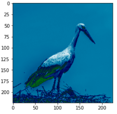
fig1: Input_image

To get the prediction vector ResNet50 will be loaded from Keras applications directly.

test_model = tf.keras.applications.resnet50.ResNet50()
#test_model.summary()
get_image()
img_path = "image.jpg"
input_img = input_img(img_path)
input_img = tf.keras.applications.densenet.preprocess_input(input_img)
plt.imshow(normalize_image(input_img[0]), cmap = "ocean")

result = test_model(input_img)
max_idx = tf.argmax(result,axis = 1)
tf.keras.applications.imagenet_utils.decode_predictions(result.numpy())

A GradientTape function is available on TensorFlow 2.x that is capable of handling the backpropagation related operations. Here, we will utilize the benefits of GradientTape to compute the saliency map of the given image.

with tf.GradientTape() as tape:
    tape.watch(input_img)
    result = test_model(input_img)
    max_score = result[0,max_idx[0]]
grads = tape.gradient(max_score, input_img)
plot_maps(normalize_image(grads[0]), normalize_image(input_img[0]))

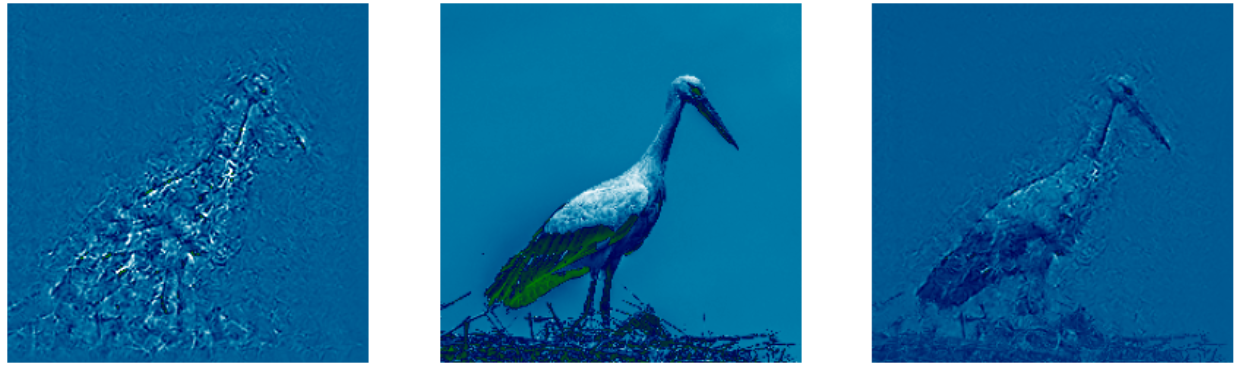
fig2: (1) Saliency_map, (2) input_image, (3) overlayed_image

Conclusion on Tensorflow 2.x

In this blog, we have defined the saliency map in different aspects. We have added a pictorial representation to understand the term “saliency map” deeply. Also, we have understood it by implementing it in python using TensorFlow API. The results seem promising and can be easily understandable.

In this article, you have learned about the saliency map for an image with tensorflow.

A python code is also implemented on an image to compute the saliency map of an image.

The mathematical background of the saliency map is also covered in this article.

That’s it! Congratulations, you just computed a saliency map.

github_repo.

The media shown in this article is not owned by Analytics Vidhya and is used at the Author’s discretion.