Image Classification Model Trained using Google Colab

Parthiban Marimuthu 21 Jul, 2022 • 5 min read

This article was published as a part of the Data Science Blogathon.

Introduction

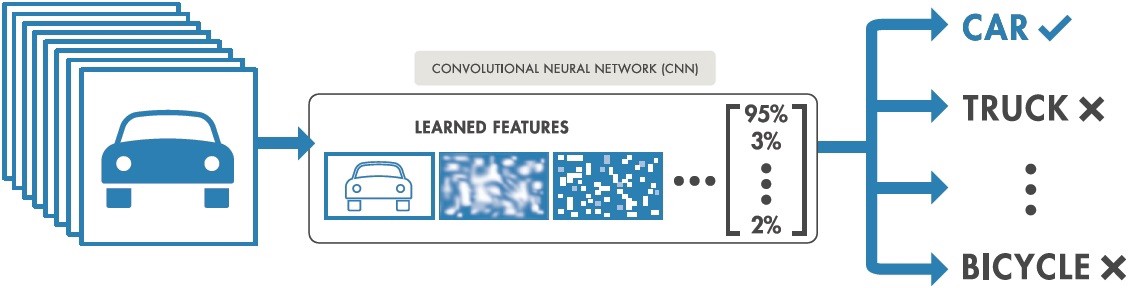
Image classification is the process of classifying and recognizing groups of pixels inside an image in line with pre-established principles. Using one or more spectral or text qualities is feasible while creating the classification regulations. Two popular types of categorization techniques are “supervised” and “unsupervised.”

^{How does Image Classification work?}

Using labeled sample photos, a model is trained to detect the target classes (objects to identify in images). An example of supervised learning is image classification. Raw pixel data was the only input for early computer vision algorithms. However, pixel data alone does not provide a sufficiently consistent representation to encompass the many oscillations of an item as represented in an image. The placement of the object, the background behind it, ambient lighting, the camera angle, and the camera focus can all affect the raw pixel data.

Traditional computer vision models added new components derived from pixel data, such as textures, colour histograms, and shapes, to model objects more flexibly. The drawback of this approach was that feature engineering became very time-consuming because of the enormous number of inputs that needed to be changed. Which hues were crucial for categorizing cats? How flexible should the definitions of shapes be? Because characteristics had to be adjusted so precisely, it was difficult to create robust models.

Train Image Classification Model

A fundamental machine learning workflow is used in this tutorial:

Analyze dataset
Create an Input pipeline
Build the model
Train the model
Analyze the model

Setup And Import TensorFlow and other libraries

import itertools
import os
import matplotlib.pylab as plt
import numpy as np
import tensorflow as tf
import tensorflow_hub as hub
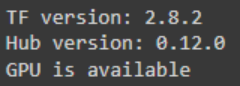
print("TF version:", tf.__version__)
print("Hub version:", hub.__version__)
print("GPU is", "available" if tf.config.list_physical_devices('GPU') else "NOT AVAILABLE")

The output looks like this:

Select the TF2 Saved Model Module to Use

More TF2 models that produce feature vectors for images may be found here. (Note that TF1 Hub-format models won’t function here.)

There are numerous models that could work. Simply choose a different option from the list in the cell below, then proceed with the notebook. Here, I selected Inception_v3 and automatically, it chose the Image size from the below list as 299 x 299.

model_name = "resnet_v1_50" # @param ['efficientnetv2-s', 'efficientnetv2-m', 'efficientnetv2-l', 'efficientnetv2-s-21k', 'efficientnetv2-m-21k', 'efficientnetv2-l-21k', 'efficientnetv2-xl-21k', 'efficientnetv2-b0-21k', 'efficientnetv2-b1-21k', 'efficientnetv2-b2-21k', 'efficientnetv2-b3-21k', 'efficientnetv2-s-21k-ft1k', 'efficientnetv2-m-21k-ft1k', 'efficientnetv2-l-21k-ft1k', 'efficientnetv2-xl-21k-ft1k', 'efficientnetv2-b0-21k-ft1k', 'efficientnetv2-b1-21k-ft1k', 'efficientnetv2-b2-21k-ft1k', 'efficientnetv2-b3-21k-ft1k', 'efficientnetv2-b0', 'efficientnetv2-b1', 'efficientnetv2-b2', 'efficientnetv2-b3', 'efficientnet_b0', 'efficientnet_b1', 'efficientnet_b2', 'efficientnet_b3', 'efficientnet_b4', 'efficientnet_b5', 'efficientnet_b6', 'efficientnet_b7', 'bit_s-r50x1', 'inception_v3', 'inception_resnet_v2', 'resnet_v1_50', 'resnet_v1_101', 'resnet_v1_152', 'resnet_v2_50', 'resnet_v2_101', 'resnet_v2_152', 'nasnet_large', 'nasnet_mobile', 'pnasnet_large', 'mobilenet_v2_100_224', 'mobilenet_v2_130_224', 'mobilenet_v2_140_224', 'mobilenet_v3_small_100_224', 'mobilenet_v3_small_075_224', 'mobilenet_v3_large_100_224', 'mobilenet_v3_large_075_224']
model_handle_map = {
  "efficientnetv2-s": "https://tfhub.dev/google/imagenet/efficientnet_v2_imagenet1k_s/feature_vector/2",
  "efficientnetv2-m": "https://tfhub.dev/google/imagenet/efficientnet_v2_imagenet1k_m/feature_vector/2",
  "efficientnetv2-l": "https://tfhub.dev/google/imagenet/efficientnet_v2_imagenet1k_l/feature_vector/2",
  "efficientnetv2-s-21k": "https://tfhub.dev/google/imagenet/efficientnet_v2_imagenet21k_s/feature_vector/2",
  "efficientnetv2-m-21k": "https://tfhub.dev/google/imagenet/efficientnet_v2_imagenet21k_m/feature_vector/2",
  "efficientnetv2-l-21k": "https://tfhub.dev/google/imagenet/efficientnet_v2_imagenet21k_l/feature_vector/2",
  "efficientnetv2-xl-21k": "https://tfhub.dev/google/imagenet/efficientnet_v2_imagenet21k_xl/feature_vector/2",
  "efficientnetv2-b0-21k": "https://tfhub.dev/google/imagenet/efficientnet_v2_imagenet21k_b0/feature_vector/2",
  "efficientnetv2-b1-21k": "https://tfhub.dev/google/imagenet/efficientnet_v2_imagenet21k_b1/feature_vector/2",
  "efficientnetv2-b2-21k": "https://tfhub.dev/google/imagenet/efficientnet_v2_imagenet21k_b2/feature_vector/2",
  "efficientnetv2-b3-21k": "https://tfhub.dev/google/imagenet/efficientnet_v2_imagenet21k_b3/feature_vector/2",
  "efficientnetv2-s-21k-ft1k": "https://tfhub.dev/google/imagenet/efficientnet_v2_imagenet21k_ft1k_s/feature_vector/2",
  "efficientnetv2-m-21k-ft1k": "https://tfhub.dev/google/imagenet/efficientnet_v2_imagenet21k_ft1k_m/feature_vector/2",
  "efficientnetv2-l-21k-ft1k": "https://tfhub.dev/google/imagenet/efficientnet_v2_imagenet21k_ft1k_l/feature_vector/2",
  "efficientnetv2-xl-21k-ft1k": "https://tfhub.dev/google/imagenet/efficientnet_v2_imagenet21k_ft1k_xl/feature_vector/2",
  "efficientnetv2-b0-21k-ft1k": "https://tfhub.dev/google/imagenet/efficientnet_v2_imagenet21k_ft1k_b0/feature_vector/2",
  "efficientnetv2-b1-21k-ft1k": "https://tfhub.dev/google/imagenet/efficientnet_v2_imagenet21k_ft1k_b1/feature_vector/2",
  "efficientnetv2-b2-21k-ft1k": "https://tfhub.dev/google/imagenet/efficientnet_v2_imagenet21k_ft1k_b2/feature_vector/2",
  "efficientnetv2-b3-21k-ft1k": "https://tfhub.dev/google/imagenet/efficientnet_v2_imagenet21k_ft1k_b3/feature_vector/2",
  "efficientnetv2-b0": "https://tfhub.dev/google/imagenet/efficientnet_v2_imagenet1k_b0/feature_vector/2",
  "efficientnetv2-b1": "https://tfhub.dev/google/imagenet/efficientnet_v2_imagenet1k_b1/feature_vector/2",
  "efficientnetv2-b2": "https://tfhub.dev/google/imagenet/efficientnet_v2_imagenet1k_b2/feature_vector/2",
  "efficientnetv2-b3": "https://tfhub.dev/google/imagenet/efficientnet_v2_imagenet1k_b3/feature_vector/2",
  "efficientnet_b0": "https://tfhub.dev/tensorflow/efficientnet/b0/feature-vector/1",
  "efficientnet_b1": "https://tfhub.dev/tensorflow/efficientnet/b1/feature-vector/1",
  "efficientnet_b2": "https://tfhub.dev/tensorflow/efficientnet/b2/feature-vector/1",
  "efficientnet_b3": "https://tfhub.dev/tensorflow/efficientnet/b3/feature-vector/1",
  "efficientnet_b4": "https://tfhub.dev/tensorflow/efficientnet/b4/feature-vector/1",
  "efficientnet_b5": "https://tfhub.dev/tensorflow/efficientnet/b5/feature-vector/1",
  "efficientnet_b6": "https://tfhub.dev/tensorflow/efficientnet/b6/feature-vector/1",
  "efficientnet_b7": "https://tfhub.dev/tensorflow/efficientnet/b7/feature-vector/1",
  "bit_s-r50x1": "https://tfhub.dev/google/bit/s-r50x1/1",
  "inception_v3": "https://tfhub.dev/google/imagenet/inception_v3/feature-vector/4",
  "inception_resnet_v2": "https://tfhub.dev/google/imagenet/inception_resnet_v2/feature-vector/4",
  "resnet_v1_50": "https://tfhub.dev/google/imagenet/resnet_v1_50/feature-vector/4",
  "resnet_v1_101": "https://tfhub.dev/google/imagenet/resnet_v1_101/feature-vector/4",
  "resnet_v1_152": "https://tfhub.dev/google/imagenet/resnet_v1_152/feature-vector/4",
  "resnet_v2_50": "https://tfhub.dev/google/imagenet/resnet_v2_50/feature-vector/4",
  "resnet_v2_101": "https://tfhub.dev/google/imagenet/resnet_v2_101/feature-vector/4",
  "resnet_v2_152": "https://tfhub.dev/google/imagenet/resnet_v2_152/feature-vector/4",
  "nasnet_large": "https://tfhub.dev/google/imagenet/nasnet_large/feature_vector/4",
  "nasnet_mobile": "https://tfhub.dev/google/imagenet/nasnet_mobile/feature_vector/4",
  "pnasnet_large": "https://tfhub.dev/google/imagenet/pnasnet_large/feature_vector/4",
  "mobilenet_v2_100_224": "https://tfhub.dev/google/imagenet/mobilenet_v2_100_224/feature_vector/4",
  "mobilenet_v2_130_224": "https://tfhub.dev/google/imagenet/mobilenet_v2_130_224/feature_vector/4",
  "mobilenet_v2_140_224": "https://tfhub.dev/google/imagenet/mobilenet_v2_140_224/feature_vector/4",
  "mobilenet_v3_small_100_224": "https://tfhub.dev/google/imagenet/mobilenet_v3_small_100_224/feature_vector/5",
  "mobilenet_v3_small_075_224": "https://tfhub.dev/google/imagenet/mobilenet_v3_small_075_224/feature_vector/5",
  "mobilenet_v3_large_100_224": "https://tfhub.dev/google/imagenet/mobilenet_v3_large_100_224/feature_vector/5",
  "mobilenet_v3_large_075_224": "https://tfhub.dev/google/imagenet/mobilenet_v3_large_075_224/feature_vector/5",
}
model_image_size_map = {
  "efficientnetv2-s": 384,
  "efficientnetv2-m": 480,
  "efficientnetv2-l": 480,
  "efficientnetv2-b0": 224,
  "efficientnetv2-b1": 240,
  "efficientnetv2-b2": 260,
  "efficientnetv2-b3": 300,
  "efficientnetv2-s-21k": 384,
  "efficientnetv2-m-21k": 480,
  "efficientnetv2-l-21k": 480,
  "efficientnetv2-xl-21k": 512,
  "efficientnetv2-b0-21k": 224,
  "efficientnetv2-b1-21k": 240,
  "efficientnetv2-b2-21k": 260,
  "efficientnetv2-b3-21k": 300,
  "efficientnetv2-s-21k-ft1k": 384,
  "efficientnetv2-m-21k-ft1k": 480,
  "efficientnetv2-l-21k-ft1k": 480,
  "efficientnetv2-xl-21k-ft1k": 512,
  "efficientnetv2-b0-21k-ft1k": 224,
  "efficientnetv2-b1-21k-ft1k": 240,
  "efficientnetv2-b2-21k-ft1k": 260,
  "efficientnetv2-b3-21k-ft1k": 300, 
  "efficientnet_b0": 224,
  "efficientnet_b1": 240,
  "efficientnet_b2": 260,
  "efficientnet_b3": 300,
  "efficientnet_b4": 380,
  "efficientnet_b5": 456,
  "efficientnet_b6": 528,
  "efficientnet_b7": 600,
  "inception_v3": 299,
  "inception_resnet_v2": 299,
  "nasnet_large": 331,
  "pnasnet_large": 331,
}
model_handle = model_handle_map.get(model_name)
pixels = model_image_size_map.get(model_name, 224)
print(f"Selected model: {model_name} : {model_handle}")
IMAGE_SIZE = (pixels, pixels)
print(f"Input size {IMAGE_SIZE}")
BATCH_SIZE = 16#@param {type:"integer"}

The inputs are scaled correctly for the selected module. A larger dataset helps with training, especially when fine-tuning (i.e., random distortions of an image each time it is read).

Our unique dataset should be organized as shown in the figure below.

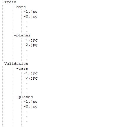
Our customized dataset must now be uploaded to Drive. We must set the data augmentation parameter to true once our dataset needs augmentation.

data_dir = "/content/Images"
def build_dataset(subset):
  return tf.keras.preprocessing.image_dataset_from_directory(data_dir,validation_split=.10,subset=subset,label_mode="categorical",seed=123,image_size=IMAGE_SIZE,batch_size=1)
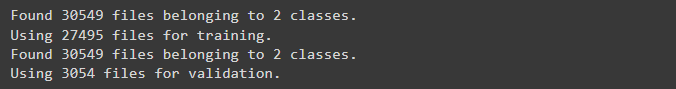
train_ds = build_dataset("training")
class_names = tuple(train_ds.class_names)
train_size = train_ds.cardinality().numpy()
train_ds = train_ds.unbatch().batch(BATCH_SIZE)
train_ds = train_ds.repeat()
normalization_layer = tf.keras.layers.Rescaling(1. / 255)
preprocessing_model = tf.keras.Sequential([normalization_layer])
do_data_augmentation = False #@param {type:"boolean"}
if do_data_augmentation:
  preprocessing_model.add(tf.keras.layers.RandomRotation(40))
  preprocessing_model.add(tf.keras.layers.RandomTranslation(0, 0.2))
  preprocessing_model.add(tf.keras.layers.RandomTranslation(0.2, 0))
  # Like the old tf.keras.preprocessing.image.ImageDataGenerator(),
  # image sizes are fixed when reading, and then a random zoom is applied.
  # RandomCrop with a batch size of 1 and rebatch later.
  preprocessing_model.add(tf.keras.layers.RandomZoom(0.2, 0.2))
  preprocessing_model.add(tf.keras.layers.RandomFlip(mode="horizontal"))
train_ds = train_ds.map(lambda images, labels:(preprocessing_model(images), labels))
val_ds = build_dataset("validation")
valid_size = val_ds.cardinality().numpy()
val_ds = val_ds.unbatch().batch(BATCH_SIZE)
val_ds = val_ds.map(lambda images, labels:(normalization_layer(images), labels))
 
Output:

Defining the Model

All that is required is to use the Hub module to layer a linear classifier on top of the feature extractor layer.

We initially use a non-trainable feature extractor layer for speed, but you can alternatively enable fine-tuning for better precision.

do_fine_tuning = True
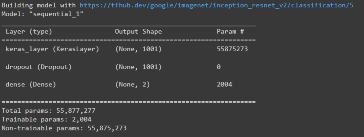
print("Building model with", model_handle)
model = tf.keras.Sequential([
    # Explicitly define the input shape so the model can be properly
    # loaded by the TFLiteConverter
    tf.keras.layers.InputLayer(input_shape=IMAGE_SIZE + (3,)),
    hub.KerasLayer(model_handle),
    tf.keras.layers.Dropout(rate=0.2),
    tf.keras.layers.Dense(len(class_names),activation='sigmoid',
    kernel_regularizer=tf.keras.regularizers.l2(0.0001))
    ])
model.build((None,)+IMAGE_SIZE+(3,))
model.summary()

Output look below

Model Training

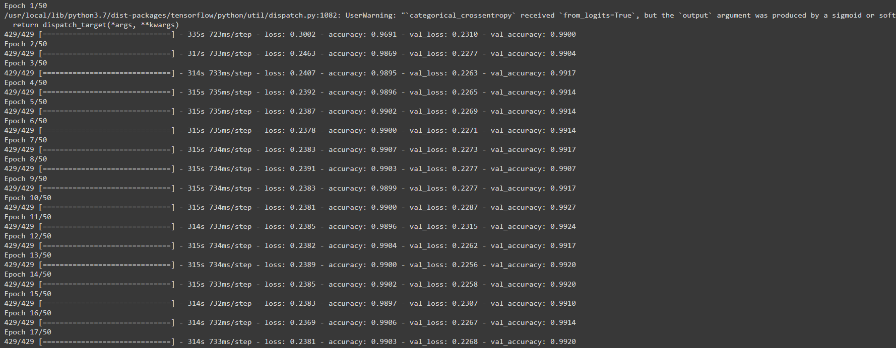
model.compile(
  optimizer=tf.keras.optimizers.SGD(learning_rate=0.005, momentum=0.9), 
  loss=tf.keras.losses.CategoricalCrossentropy(from_logits=True, label_smoothing=0.1),
  metrics=['accuracy'])

steps_per_epoch = train_size // BATCH_SIZE

validation_steps = valid_size // BATCH_SIZE

hist = model.fit(

train_ds,

epochs=50, steps_per_epoch=steps_per_epoch,

validation_data=val_ds,

validation_steps=validation_steps).history

The output looks below:

Once training is completed, we need to save the model by using the following code:

model.save ("save_locationmodelname.h5")

Conclusion

This blog post categorized pictures using convolutional neural networks (CNNs) based on their visual content. This data set was utilized for testing and training CNN. Its accuracy percentage is greater than 98 per cent. We must employ tiny, grayscale images as our teaching resources. These photos require a pervasive processing time compared to other regular JPEG photos. A model with more layers and more picture data used to train the network on a cluster of GPUs would classify images more accurately. Future development will concentrate on categorizing enormous coloured images that are very useful for the segmentation process of images.

Key Takeaways

Image classification, a branch of computer vision, classifies and labels sets of pixels or vectors inside an image using a set of specified tags or categories that an algorithm has been trained on.
It is possible to differentiate between supervised and unsupervised classification.
In supervised classification, the classification algorithm is trained using a set of images and their associated labels.
Unsupervised classification algorithms only use raw data for training.
You require a sizable diversity of datasets with accurately labelled data to create trustworthy picture classifiers.

Thanks for reading!

The media shown in this article is not owned by Analytics Vidhya and is used at the Author’s discretion.

3D-CNN Model image classification. blogathon

Parthiban Marimuthu 21 Jul 2022

Beginner Computer Vision Deep Learning Image Analysis Python