Job interviews can be scary if you are a fresher and especially if you are attending interviews on interdisciplinary roles like Data Science and Machine Learning. The tension, the doubt if you will get a yes or a no at the end of the interview, and whether you can answer all that you are asked, properly, can lead to distraction during preparations. So here in this article, I will be sharing some of the most encountered questions from various subjects under Data Science and ML/AI, from my previous interview experiences.
Although these are the most repetitive ones, you may or may not get these asked. Questions often depend on the kind of work done in the company or organization (for example — if the organization doesn’t deal with time-series data, you will not be getting time-series questions).
Note – No matter what, these 15 curated questions must be at your toung tip before attending any data science interview!
Without further ado, let us get to the subject!
15 Important Data Science Interview Questions
1. What is a Confusion Matrix? Describe its role in your own words. What do you understand by Type I and Type II errors?
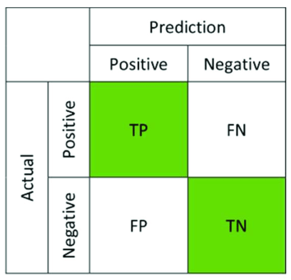
Ans. In real-world machine learning, a confusion matrix is a very useful way to summarize a machine learning model’s performance. The idea behind the confusion matrix directly came from the perception that it is not a great idea to judge a classification task only by its accuracy. Imbalanced data is biased/skewed and hence gives wrong classification results.
A confusion matrix, thus, provides a better way to check a model’s performance. A confusion matrix is a 2×2 matrix consisting of 4 key metrics – true positive, false positive, true negative and false negative.
True positive (TP) – Correct predictions of true events
False positive (FP) – Incorrect predictions of true events. Also called Type-I error.
True negative (TN)- Correct predictions of false events
False negative (FN)- Incorrect predictions of false events. Also called Type-II error.
A model can be well judged by 3 metrics called sensitivity, specificity and accuracy, which can be calculated from a confusion matrix.
Sensitivity – It is the measure of correctly predicted proportions of true positives.
Formula – TP/(TP + FN)
Specificity – It is the measure of correctly predicted proportions of true negatives
Formula – TN/(TN + FP)
Accuracy – Measures the degree of veracity in a classification. It is simply the proportion of all true predictions ( TP and TN).
Formula – (TP + TN)/(TP + TN + FP + FN)
Source – ResearchGate
2. Define precision, recall, and f1-score with their formulas.
Ans. Precision — Precision is the measure of the proportion of true positives to the total number of predicted positives. It helps to analyze the quality of prediction, and higher precision means a model is generalized and gives almost correct results.
Formula — TP/(TP+FP)
Recall — Also called Sensitivity/True Positive Rate (TPR)/Probability of Detection, recall is the ratio of true positives to the total positives. It helps to measure the true positive rate and completeness of prediction.
Formula — TP/(TP + FN)
F1 score — The weighted harmonic mean between Precision and Recall is the F1 Score. It takes both Precision and Recall to rate a model’s performance.
Formula — 2 x (Precision x Recall)/(Precision + Recall)
3. How would you distinguish feature selection and feature extraction?
Ans. Feature Selection and Feature Extraction are two very important techniques to scale down high dimensional data to solve the Curse of Dimensionality (too many features which may not be necessary, and hinders good modelling).
Feature Selection — It is a known fact that an increase in input feature variables can consume computational resources, and slow down modelling, which leads to overall failure. Feature Selection is that stage of data preprocessing where only the features essential to predict the target are considered for modelling, and the irrelevant and redundant features are removed. This is the stage on which the robustness of the ML pipeline to be developed later on depends, and hence plenty of time and effort should be given to this stage. An optimized feature set can lead to easier modelling, fast computation, robust machine learning pipeline which can be easily scaled and ready for production.
Feature Extraction — Feature Extraction is a process which accelerates proper feature selection to a great extent. Feature extraction takes the task of transforming features from existing data to extract new features. Feature extraction (transformations) should be done before feature selection, as feature selection depends right on top of extracted features.
So, in the data preprocessing stage, features are extracted from given data (like n-grams/ parts of speech tags from text, corners/edges from images) by transforming the data. Further, feature selection is done to remove irrelevant and redundant features, and finally, data-mining (exploring trends and insights from data) and modelling (interpretation and evaluation) are performed.
4. What do you know about Autoregression and Moving Average? Why we cannot take non-stationary data to solve time series problems?
Ans. Generally used as a statistical tool to work with time-series data, Autoregression is a technique which uses regression (generally linear regression) to take input/lag variables (observations at previous time steps, hence autoregression) and models them to output the target variable at a future time step, based on a linear combination of lag variables.
Let’s mathematically explain this –
X(t+1) = b0 + b1 * X(t-1) + b2 * X(t-2),
where b0,b1 = coefficients calculated by optimization of training dataset
X(t+1) = predicted value at timestamp (t+1)
X(t-1) , X(t-2) = input variables/observations at previous timestamps (t-1) and (t-2)
A Moving Average is simply calculated means over a changing subset of numbers (sliding window in mathematical terms). In time-series data, we use this extremely helpful technique of calculating averages of a particular time-variant feature over certain periods.
For example, in stock market forecasting, IT giants use moving averages to see stock trends in the market, in periods, which helps them forecast where their stocks will be headed for the next 2–3 months or so on.
Also, interchangeably called Rolling Mean, here is what it does –
Let the mean at timestamp t-1 is x and t-2 be y, so we find the average of x and y to predict the value at timestamp t+1. The sliding window hence takes a mean of 2 values to predict the 3rd value. After it is done, it will slide to the next subset of values.
Source – Wikipedia
The moving average model, instead of taking in values at previous time steps, takes lagged forecast errors in previous values (white noise error) to predict the ultimate forecast.
Part II –
We cannot take non-stationary data to solve a time-series problem. NEVER.
Generally, stationarity means non-fluctuation and consistency. Any machine learning model will perform well when the data it is fitting is stationary in nature, i.e. without high fluctuations (no consistency in input/output parameters like mean, median, variance).
In time-series forecasting, the data is highly fluctuating, as with time periods, comes seasonalities and trends, which tend to make the data sharply inconsistent. It is impossible to model the data with such highly fluctuating mean and variances. Forecasting meets crisis.
So, it is extremely crucial to check stationarity and remove non-stationarity (if any) from the data before modelling it.
5. Explain Hidden Markov Model. Why is it called ‘Hidden’?
Ans. Hidden Markov Models are just Markov Models with hidden states. HMMs are specially used to solve problems using Machine Learning where a “hidden” target is predicted based on a set of “observed” features/attributes. For example, your “mental health” which is a hidden state, can be predicted by a set of observed features like { sleep hours, stress levels, work pressure, physical health, trauma/abuse }.
A Hidden Markov Model has the following probabilistic parameters –
y(i) – i number of observations (y)
X(i) – i number of states (X)
a – transition probability of states
b – output/emission probability
Using these parameters, the HMM tries to answer the question –
“What is the likelihood or how much likely it is for the observation y(i) to happen?“
Based on the emission or output probability that we get, we can easily decide whether it is likely to happen (close to 1) or not (far behind 1).
In a Hidden Markov Model, probabilistic inferences “hidden target” are drawn based on maximum likelihood estimations, of a Markov process which relies on the principle that “given the present, the future is always independent of the past”. Hence, the name, Hidden Markov Model.
6. What do you know about Autoencoders? Are they similar to PCA?
Ans. Autoencoders are a type of Artificial Neural Network architecture belonging to the wide and diverse family of ANNs. The uniqueness of Autoencoders is that it is a feature-learning algorithm that produces the same output as input, unlike other neural networks which output a probability distribution of classes.
NOTE — Autoencoders work on a mechanism of data compression, which is conventionally said to be latent space representation by stacking multiple non-linear transformations(layers). Latent means “hidden”. When you classify a dog and cat by images of both, the machine, in the first place, is able to point out a dog and a cat by learning facial features or in machine-learning terms, structural similarities from images. But do we really get to see how this process works? Nope. Hence, we call it Latent Space Representation or, in simple words, Hidden Space Representation.
So, the task of Autoencoders is to compress the input data into latent space representations (used to extract feature similarity as similar features in images will lie as coordinates close to each other in latent space) to extract feature similarities, and finally reconstruct (using upsampling and convolution operations) the output image all by itself.
Compression is a go-to word for dimensionality reduction. Compression is heavily used in Deep Learning to reduce the dimensionality of images by removing the irrelevant details and focusing on the relevant ones only. It is generally done by encoding the n-dimensional data to 1 dimensional and then decoding it to produce the original one.
Although Autoencoders resembles PCA, yet it is considered to be better than PCA in cases where non-linear feature spaces in present (PCA can only handle linear transformations, and using it on non-linear spaces will lead to loss of relevant information).
Autoencoders are really useful in reducing the dimensionality of high-dimensional image data, which comes at an expensive computational cost while carrying out computer vision tasks. One of the numerous compression benefits that autoencoders have, is removing noise and outputting clear data.
7. What is vanishing and exploding gradients?
Ans. During model training, stochastic gradient descent (or SGD) computes the gradient of the loss function with respect to weights in the neural network. During backpropagation (calculation of gradients) we update functional parameters (weights) to minimize that lost function, by the chain rule of differentiation (product of some derivatives that depend on parameters that reside later in the network). Now, sometimes the gradient with respect to weights in previous layers of the network starts becoming smaller and smaller WRT time and finally squashes to 0.
VANISH!!
Hence, the vanishing gradient. (Well, the product of a bunch of numbers less than 1 is going to give us an even smaller number. And subtracting such a small quantity from the weight would never really update the weight. Pretty self-explanatory.)
Exploding Gradient is the ‘Upside Down’ of Vanishing Gradient. Suppose our gradient value is a large number, say 1. So, the product of a bunch of numbers greater than 1 is going to give us an even greater number. And hence, there is a huge change in weights at each epoch which results in large values, and therefore it moves away from the optimal value, resulting in the explosion of the gradient.
8.Explain Tokenization, Stemming and Lemmatization in NLP text preprocessing.
Ans. Tokenization is a very basic text preprocessing stage where large sentence pieces in text corpora are broken down into their smallest unit, that is words (often sentences), which are represented as tokens. Tokenization is important in text mining and processing to compute word frequencies, which are required during modelling.
Tokenizers are generally of two types –
Word level tokenizer — Breaks down the text to word level.
Syntax : tokenize.word_tokenize()
Return Type : Returns list of words.
Sentence level tokenizer — Breaks down the text to sentence level.
Syntax : tokenize.sent_tokenize()
Return Type : Returns list of sentences.
Stemming or Rooting is another text preprocessing technique where words are reduced to their base level or root level (for example, word = ‘stems’, root = ‘stem’) to avoid different grammatical forms of the same word in the processed text.
Though stemming works fine, for some words, it may give weird and nonsense outputs, like it gives the base as ‘strok’ for the word ‘stroking’. ‘strok’ is not even a word, and we lost the correct data ‘stroking’ we had. If this process happens a lot in the text fed to the stemmer, a lot of information will be lost, resulting in model failure later.
Lemmatization was developed to address the loophole spotted in stemming that we just saw. It takes care of the derivational affixes and doesn’t lose the original word, as it returns exactly the dictionary base of a word, called ‘lemma’. Lemmatization works in a more logical approach by keeping into account the parts of speech and morphology of the text.
For example, if we feed ‘United’ and ‘States’ to Stemmer, we get ‘Unite’ and ‘State’, whereas the lemmatizer understands from parts of speech that it is a proper noun (has ‘the’ before it) and returns ‘United’ and ‘States’ without altering the original form.
9. Briefly explain the role of the TFIDF algorithm in solving NLP use cases.
Ans. TF-IDF is short for Term Frequency Inverse Document Frequency. It is an information retrieval algorithm that assigns a score or weight factor to documents present in a text corpus to be used to carry out NLP use cases. Scoring directly helps in understanding how important words or sentences are, which in turn helps in eliminating extraneous/irrelevant vocabularies from the corpora and focuses more on important or highly scored words/sentences.
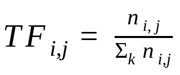
TF-IDF is computed using two kinds of frequency. Term Frequency(TF) and Inverse Document Frequency(IDF).
Term Frequency (TF) — It is just the frequency of terms (words) present in the document. For large texts, the TF value may be very high for some words, hence normalization of TF is done by dividing the frequency of a word (w) found in the document by the total number of words in the document.
Inverse Document Frequency (IDF) — IDF assigns a higher score or simply weightage to terms/words that are rarely found in the document. The rarer the term, the higher the IDF weightage or score.
Note — IDF calculation (degree of uniqueness) is important because, when the document’s length increases, words like ‘as’, ‘therefore’, ‘since’, ‘there’, ‘then’, ‘that’, etc, increases to a large extent. These words really do not contribute more to the machine learning part, and hence rare words or document-specific words which occur less (but important) are scored higher by IDF. For example, it helps search engines give really good results by checking the unique words entered in the search and not frequent terms.
IDF is calculated by taking the log of the ratio of the total number of documents to the number of documents with the term ‘t’ in it.
Thus, TFIDF is nothing but product of TF and IDF –
TFIDF = TF * IDF
10. What is Central Limit Theorem? Do you accept or reject the Null Hypothesis? Explain with valid points.
Ans. The Central Limit Theorem simply states that, if we have a population data given, be it any kind of distribution with finite mean and variance/standard deviation, then the sampling distribution of the sampling means will always be a Normal/Gaussian distribution.
A Null Hypothesis, as the name suggests, can either be nullified or rejected.
Let’s suppose you think you have been attacked by Corona Virus, and thus you’re Covid Positive. What they assume is what we call a Null Hypothesis. The alternate hypothesis — the one you want to replace with the null hypothesis, is that you aren’t covid positive. So, you would want to reject the null hypothesis — prove that you are not covid positive.
Note — You either reject the null hypothesis or fail to reject the null hypothesis.
The null hypothesis is the hypothesis to be tested.
Failing to reject the null means that there isn’t enough data to support the change or the innovation brought by the alternative. To reject the null means that there is enough statistical evidence that the null hypothesis is not representative of the truth.
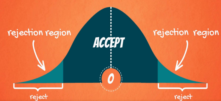
Let us look at a visual representation –
Source – 365DataScience
Given a two-tailed test above:
Graphically, the tails of the distribution show when we reject the null hypothesis (notice ‘rejection region’). Everything which remains in the middle is the ‘acceptance region’.
The rationale is that if the observed statistic is too far away from 0 (depending on the significance level), we reject the null. Otherwise, we accept it.
To calculate significance levels (probability of rejecting a null hypothesis that is true), we need to calculate p-values. A p-value is the smallest level of significance at which we can still reject the null hypothesis, given the observed sample statistic.
Some important characteristics of p-values –
usually found with 3 digits after the dot (x.xxx).
closer to 0.000 the p-value, the better it is.
There are two types of notable p-values (significance level — alpha). The trick to doing hypothesis testing is as follows –
0.000 — When we are testing a hypothesis, we always strive for those ‘three zeros after the dot’. This indicates that we reject the null at all significance levels.
0.05 — It is the “threshold” of the p-value. ’. If our p-value is higher than 0.05 we would normally accept the null hypothesis (equivalent to testing at 5% significance level). If the p-value is lower than 0.05 we would reject the null. If it is exactly 0.05, you can decide either way.
11. Compare and contrast L1-regularization vs. L2-regularization.
Ans. Regularization is the most common way of controlling the model’s complexity and reducing overfitting in a flexible and tunable manner.
L1 regularization or L1 norm or Lasso Regression works by squashing the model-specific parameters towards 0. In simple words, what L1 Regularization does is, assigns a value of 0 to feature weights which do not contribute much to the predictive ability of the machine learning model. Hence, it works like a feature selection approach.
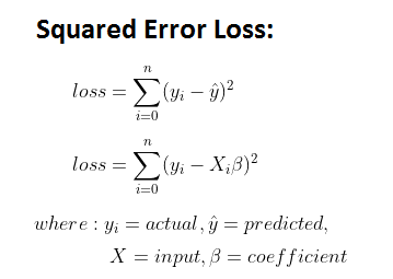
We simply do this by adding on a penalty term to the loss function we have in Generalized Linear Models (Regression, for example) –
We know that the squared loss is –
Now Regularization simply adds on a penalty term to penalize |weight| (Wj) by forcing the irrelevant features to be of 0 weight. The formula is as follows –
The formula is no rocket science stuff. It’s just a penalty term added to the Residual Sum of Squares (RSS) formula. The lambda hyperparameter (regularization rate) tunes the amount of regularization applied to the model. The larger lambda is, the more the coefficients are shrunk toward zero, and the model may underfit.
So, Lasso or L1 regularization adds the absolute value of the coefficient to the error term. Thus, this regularization term contributes to optimal feature selection by discarding them, when we have too many features to choose from in predictive modelling.
L2 regularization or L2 norm or Ridge Regression works similarly except for the penalty term where instead of taking absolute values of the coefficients, we take squared values of them.
The formula for L2 regularization is as follows –
What differentiates it from L1 is that it forces coefficients/weights towards 0, but never makes them equal to 0. The regularization rate, again, lambda, is used to control the rate of penalization of the regularization element.
Note — The higher the lambda, the complexity will decrease more, and model underfits. The lower the lambda, complexity increases and overfitting occurs. So hyperparameter tuning of lambda needs to be done very carefully to ensure robust performance of model.
12. Why are ensemble methods superior to individual models?
Ans. Ensemble Methods are a class of Machine Learning algorithms that combine several machine learning algorithms ( collectively called weak learners) and stack them to form an ensemble learner (strong learner) by combining predictions of various weak learners into one supervised model. They are known to be of 3 types –
Bagging
Boosting
Stacking
Ensemble techniques are proven to be much superior to individual models when solving a complex problem with Machine Learning. Ensemble approaches like bagging can reduce variance, boosting can control bias and stacking can improve predictions to a great extent.
Bagging — Also known as Bootstrap Aggregation, Bagging is the ensemble method which is extensively used to work on reducing the variance of noisy data and helps in reducing signs of overfitting.
For example — Fitting many Decision Trees on random and different samples of the same dataset and averaging the predictions made by each sample (just like divide and conquer), thus making the model more stabilized and robust. This helps in reducing overfitting by greatly dealing with the bias-variance tradeoffs.
Boosting — Boosting works on ‘boosting’ the strength by working on the ‘weaknesses’. Boosting applies an ensemble learning approach to train a sequence of base models called ‘weak learners’, where each learner compensates for the weakness of its precursor. It works on the idea “United we stand, divided we fall.” Thus, bagging strictly focuses on correcting prediction errors.
Stacking — Stacking basically stitches up the performances of multiple classification/regression models, and thus can produce great predictions that no other individual model can. In stacking, every single model takes the job to learn the best combinations of predictions done by its co-workers. The stacking process consists of Base Models followed by a Meta Model. The base models fit themselves on the training data and predict outputs, which are altogether compiled. The meta-model then learns how to best combine the predictions of the base models.
Ensemble Models are ranked above individual ML models due to their –
1. Performance—An ensemble can make better predictions and achieve better performance than any single base model.
2. Robustness—An ensemble reduces the variance of the predictions and model performance, and controls overfitting.
3. Stability—Great for dealing with a bias-variance tradeoff. Bagging is used when there is low bias—high variance and boosted when there is high bias—low variance.
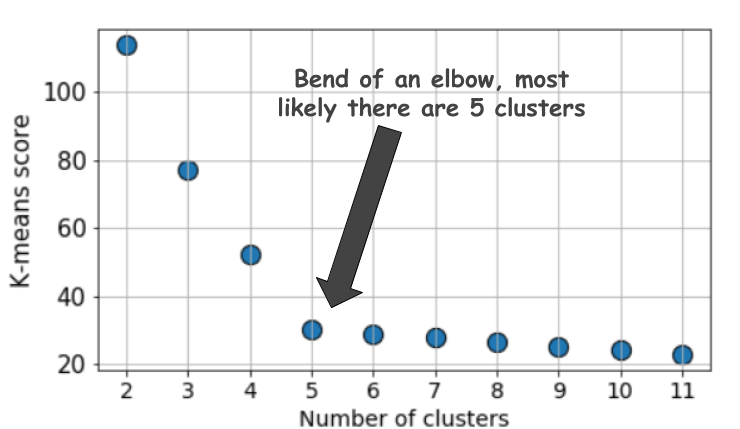
13. What is the significance of the Elbow method in K Means Clustering? According to your opinion, does Elbow Method always give an optimal number of clusters?
Ans. Elbow Method is the most standardized approach to calculating the optimal number of clusters in the unsupervised learning process of the K-Means Clustering algorithm. The steps to calculate the optimal number of clusters through the Elbow Method are quite straightforward and simple –
Try on expected values of k ( from 1 to 10).
For each value of k, we calculate the WCSS (Within Cluster Sum of Square) score.
Then the WCSS* scores are plotted against the values of k. The resulting plot is supposed to look like an elbow. (explained below)
The Elbow point is plotted to be the best/optimal k value.
WCSS* or Within-Cluster-Sum of Squared Errors sounds a bit complex. Let’s break it down:
3.1. The Squared Error for each point is the square of the distance of the point from its representation i.e. its predicted cluster center.
3.2. The WCSS score is the sum of these Squared Errors for all the points.
3.3. Any distance metric like the Euclidean Distance or the Manhattan Distance can be used.
Note — As the number of clusters increases, the WCSS metric will start to fall down. WCSS is largest when k = 1.
According to my opinion, the Elbow Method is a bit naive in its approach. Often, the elbow is not exact or steep enough to choose the optimal k, and it may be confusing as many values seem to be found in the elbow region, whereas, only one is expected to be found there.
Source – Medium
From this plot, we really cannot decide what k could be, 4, 5 or 6? A trial and error can still work, but often it doesn’t – when the elbow region itself is not found (does not mean there are no optimal clusters for our problem!).
14. After analyzing the model, your manager has informed you that your regression model is suffering from multicollinearity. How would you check if he’s true? Without losing any information, can you still build a better model?
Ans. First things first, multicollinearity is an aesthetic way of saying that the independent variables or features in the dataset are highly correlated with each other. Multicollinearity may be a serious issue as it disrupts the ‘independent’ nature of independent variables, makes it hard to interpret your coefficients, and reduces the power of your model to identify independent variables that are statistically significant. It is very self-explanatory that if variables are highly correlated with each other, then a change in one variable would cause a drastic change in the other and so the model results will fluctuate significantly, making it non-stationary. The model can collapse!
So, I need to check if the features in my dataset are highly correlated or not. Multicollinearity can be checked by –
1. Standard Practice — Plot a correlation matrix right during the exploratory data analysis. It will show the pairwise correlation coefficients between different independent variables, so you can spot multicollinearity. A bit of a time-consuming task it is, though.
2. Variation Inflation Factor (VIF) — Takes less time and more sophisticated practice. VIF is calculated for each independent variable using the R squared value (VIF = 1/1-R²). It measures the correlation of one independent variable with all the rest of the independent variables present in the dataset. The greater the value, the more multicollinearity. Most of the research concludes that a VIF > 10 means there’s serious multicollinearity and that less than 4 means there’s no multicollinearity.
3. For categorical and continuous data at hand, use the ANOVA test to check multicollinearity. However, if they aren’t continuous, Spearman Rank Correlation Coefficient or Chi-Squared Test is enough.
Removing independent variables with multicollinearity is a very bad idea, as they may be good predictors. Discarding them can lead to the loss of important information. So it is better to treat multicollinearity by taking the below methods into practice –
1. Performing an L1 / L2 norm (Ridge or Lasso Regression) as it has weight penalizers that reduces multicollinearity by shrinking the coefficients of the features that are multicollinear.
2. If your data has categorical variables, one hot encoding scan often arise the chances of multicollinearity. An effective way to remove them is by setting drop_first=True in the pd.get_dummies() function. It is seen to handle multicollinearity.
These processes can help extensively to build better models without losing any information!
15. What is Scalability in MLOps? What is the goal of MLOps? What are your experiences and ideas on the scalability of ML pipelines?
Ans. “Machine Learning is more than training the best model”
The successful production of any AI/ML pipeline must ensure scalability. Scalability in MLOps is designing a large-scale model that can handle a large amount of data fed to it in very less time in a cost-efficient way, without consuming too much memory or CPU, and work smoothly for millions of users throughout the world at good speed and accuracy.
The goal of MLOps is very straightforward –
Faster experimentation and model development
Faster deployment of updated models into production
Containerization, orchestration, and large-scale distribution of ML applications
Accelerating and scaling ML workloads for large-scale ML models is very crucial for managing and processing large quantities of data, selecting optimized and efficient machine learning algorithms, deploying the models to production, monitoring their performances on new data, and re-constructing them if necessary.
My ideas on scaling ML workloads are as follows –
1. Amazon Sagemaker — The one-stop solution for fast, cost-efficient, scalable and secure development, training and deploying ML pipelines at scale. With a one-click training environment, highly-optimized machine learning algorithms with built-in model tuning, and deployment without engineering effort, life is really less hectic in the cloud! Your ML pipeline is now absolutely production-ready, whether it is a batch prediction or real-time!
2. Use FLASK to develop the machine learning application. Flask will make you stay away from the panic of developing the application source code and help you a lot to focus on building the best possible ML solution, feature engineering, data analysis and other crucial tasks. I really love the simplicity of Flask in creating data-driven, scalable web applications in very few lines of code!
3. TensorFlow Serving –
TensorFlow Serving is a flexible, high-performance serving system for machine learning models, designed for production environments. TensorFlow Serving makes it easy to deploy new algorithms and experiments, while keeping the same server architecture and APIs. — TensorFlow
Head over here to see the documentation in detail!
4. Ensure environment friendliness in your ML pipeline by containerizing it –
Docker containers make it easy to make your code run smoothly across different environments and operating systems. All kinds of environmental dependencies are handled by docker itself. It may save you hours of frustration and will help in easier teamwork, while you and your teammates are using different virtual environments for working.
Tips for your Data Science Interview
To ace your interview you must –
1. Prepare the basics of statistical modelling.
2. Have the product sense of the company where you will be interviewed. (the kind of analytics they do, the kind of data and business problems they work on)
3. Practice implementing ML techniques/algorithms before interview. Spend atleast 2 hours a day on thoroughly studying Kaggle top voted notebooks by searching topics with a simple keyword search.
4. Pick problem statements from various Kaggle competitions and try to solve them (remember it is perfectly fine to view what others did and take ideas, but make sure you code your notebook all by yourself!)
5. Brush up your SQL and Python coding skills.
6. The R2 rule (I made it up myself and it works everytime) – It’s not the coefficient of determination though, but be determined enough to Revise and Review every project you put in your resume. No matter how well you remember implementing them, a revise on the code and recalling the challenges you faced and how you solved them, what you learnt on your journey throughout the project is very necessary as a LOT of grueling questions will be asked on your personal projects.
and lastly,
7. Stay true to yourself and do not try to make up answers to things you don’t know. Just humbly say you really don’t know the answer to that but you surely will work on it! HELPS A LOT!
Conclusion
Cheers on reaching the end of this article! Hope this article will help you ace your data science interviews.
Your key takeaways from this article are-
1. You had a quick revision on important data science stuffs like Central Limit Theorem, L1/L2 Regularization, vanishing/exploding gradients and so on.
2. Tips for your data science interview.
All the best!
If you like this article on data science interview questions, make sure to follow me on LinkedIn for more discussions on Data Science and ML! Head over to my GitHub and Medium for more contents on Data Science.
The media shown in this article is not owned by Analytics Vidhya and is used at the Author’s discretion.
An ace multi-skilled programmer whose major area of work and interest lies in Software Development, Data Science, and Machine Learning. A proactive and detail-oriented individual who loves data storytelling, and is curious and passionate to solve complex value-oriented business problems with Data Science and Machine Learning to deliver robust machine learning pipelines that ensure maximum impact.
In my free time, I focus on creating Data Science and AI/ML content, providing 1:1 mentorships, career guidance and interview preparation tips, with a sole focus on teaching complex topics the easier way, to help people make a successful career transition to Data Science with the right skillset!

.png)
.png)

.png)
.png)