This article was published as a part of the Data Science Blogathon.

Introduction
An interview process for roles like machine learning engineer and/or data scientist positions often includes multiple rounds. These rounds tend to access the candidate’s theoretical and practical concepts brutally. An important point to note here is that most tech giants prefer candidates who know how to develop robust machine-learning pipelines and how those machine learning algorithms work under the hood!
In this article, I will pen down some of the medium-to-hard yet fundamental machine-learning concepts frequently asked in machine-learning and data science interviews.
In a nutshell, while preparing for your machine learning interviews, make sure these questions are not skipped at all!
Let’s begin!
Advanced Machine Learning Interview Questions
Q1. While analyzing your model’s performance, you noticed that your model has low bias and high variance. What measures will you use to prevent it (describe two of your preferred measures)?
A: In a nutshell, Bias is nothing but the error gained from training data, and variance is the error gained from testing data. Low bias means the training error is low, and high variance means our testing error is high. This kind of bias-variance trade-off occurs when the training samples are very high, and the model learns even the random fluctuations (noise), thereby fitting too closely to the training data. This reduces the robustness and generalization capacity of the model, leading to performance failure.
Thus, overfitting, aka low bias and high variance can be prevented by the following ideas-
1. Regularization (the most standardized way)
A. L1 Regularization — L1 regularization or L1 norm or Lasso Regression works by squashing the model-specific parameters towards 0. In simple words, what L1 Regularization does is, assigns a value of 0 to feature weights that do not contribute much to the predictive ability of the machine learning model. Hence, it works like a feature selection approach.
We do this by adding a penalty term to the loss function we have in Generalized Linear Models (Regression, for example) –
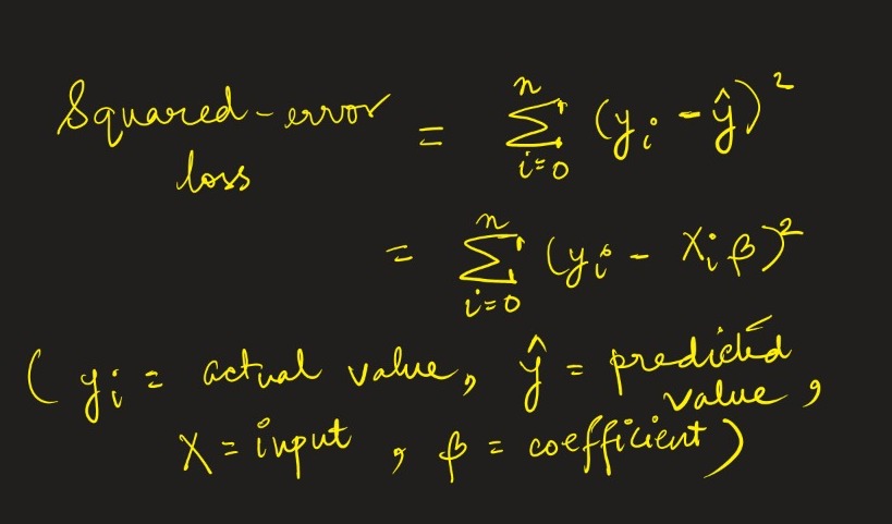
We know that the squared loss is –
Now, Regularization introduces a penalty term to penalize |weight| (Wj) by forcing the irrelevant features to be of 0 weight. The formula is –
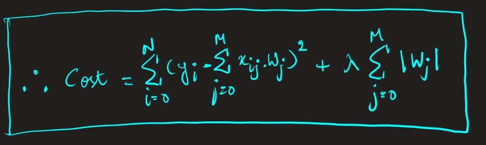
The formula is no rocket science stuff. It’s just a penalty term added to the Residual Sum of Squares (RSS) formula. The lambda hyperparameter is the rate at which we regularize. It tunes the amount of regularization applied to the model. The larger lambda is, the more the coefficients get shrunk toward zero, and the model may underfit.
So, Lasso or L1 regularization adds the absolute value of the coefficient to the error term. Thus, this regularization term contributes to optimal feature selection by discarding them, when we have too many features to choose from in predictive modeling.
L2 regularization or L2 norm or Ridge Regression is similar except for the penalty term where instead of taking absolute values of the coefficients, we take squared values of them.
The formula for L2 regularization is –
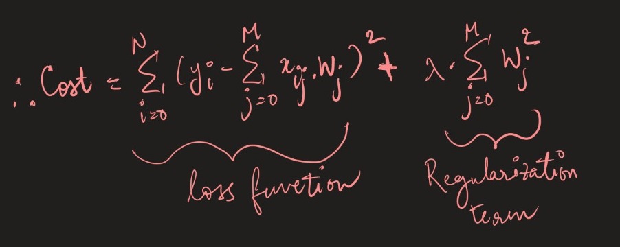
What differentiates it from L1 is that it forces coefficients/weights towards 0 but never makes them equal to 0. The lambda is used to control the penalization of the regularization element.
The higher the lambda, the complexity will decrease more, and the model underfits. The lower the lambda, complexity increases, and overfitting occurs. So tuning of lambda needs to be done very carefully to ensure the robust performance of the model.
2. Ensemble Models (the coolest way)
Bagging Method (random sampling with replacement)-
A viral algorithm called Random Forests is known to use the concept of bagging. Bagging (Bootstrap Aggregating) can be used to reduce the variance in model predictions. In bagging, numerous samples of the original data set are created using random sampling with replacement. Each sample data set is then used to construct a separate decision tree, and the models are gathered together into an ensemble (random forest). Finally, all the decision trees’ predictions are compared and aggregated or averaged to give the final prediction.
In random forests, none of the samples is seen while the decision trees/ base learners are trained (as they are trained independently). This is incredibly helpful in avoiding that unwanted data leakage and lowering the variance, thereby reducing overfitting. Multiple decision trees sum up to a “forest”, and then by averaging them, the variance of the final model can be greatly reduced over that of a single tree.
Q2. What will you do if your ANN’s (Artificial Neural Network) training loss is not updated?
A: 1. Training loss fails to update when the weights are not updated during backpropagation in the neural network. A weight update needs to be done for the model to reach the global minimum. That will ensure that the model’s loss function is minimized.
The learning rate hyperparameter needs to be tuned properly to make the weights update. Setting the learning rate at a slightly higher value often noticeably updates the weights during backprop.
2. Try using optimizers (Adam, or RMSProp). Optimizers tweaks the hyperparameters of your neural network such as weights and learning rate to reduce the losses.
Q3. How will you implement dropout during forward and backward passes?
A: Dropout is the traditional and most efficient way to regularize neural networks in order to avoid overfitting (failing to give correct predictions on unseen data due to memorizing seen data -details discussed in Q1). What dropout does is very simple. No rocket science.
Dropout means switching off random, artificial neurons during the training phase. When I say “switching off”, by a probability ‘p’, what I mean is these units are ignored during some of the backpropor frontprop. Dropout is an elegant way to perform regularization in neural networks, thereby lowering the interdependency amongst the learning neurons.
Let’s catch the concept mathematically-
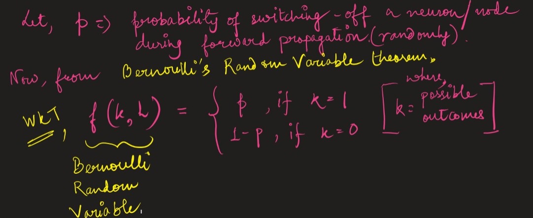
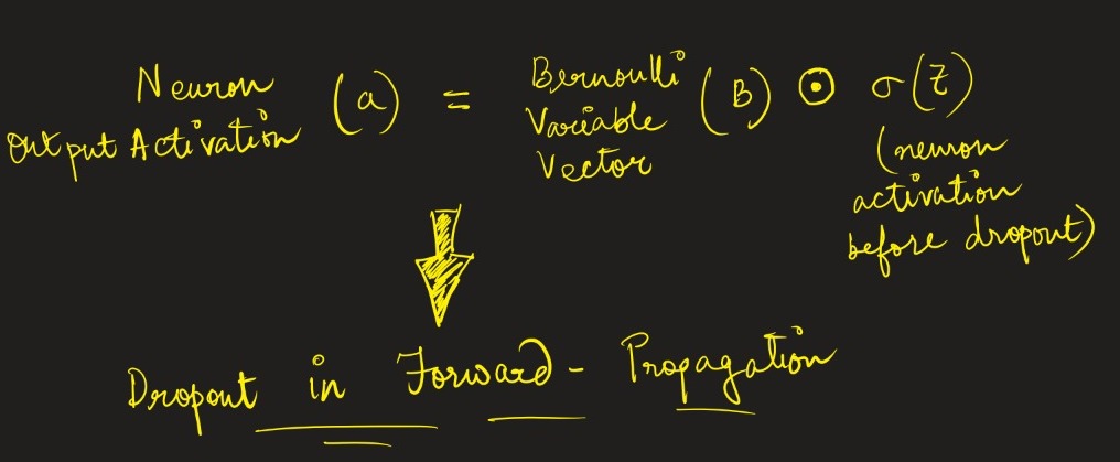
During front propagation, say if a random neuron or node is switched off by probability ‘p’, then from Bernoulli’s random variable, we can deduce the following –
Hence, what dropout internally does during the training phase is it no longer contributes any further towards learning during both forward and backward propagation when the output of the neuron is scaled to 0.
However, we cannot drop any units (neurons) during the testing phase. Hence, to match the expected value at training, we use inverted dropout, where inverse scaling is applied at the training phase. As discussed earlier, first, we dropout all activations by dropout factor p, and second, scale them by inverse dropout factor 1/p. Inverted dropout ensures that the network is left alone during the testing phase.
Thus, dropout during front propagation can be given as –
Implementation –
mask = np.random.binomial(1,p,size=X.shape) / p
out = X * mask
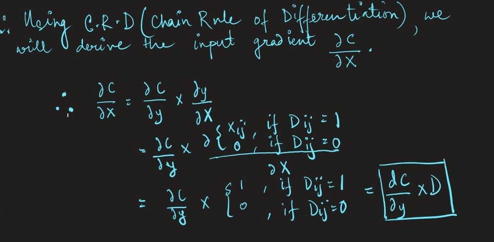
During backpropagation, we backpropagate and update the weights of the gradients with the nodes or units which weren’t turned off during the forward pass.
Implementation –
dX = dout * mask
Q4. What is a hyperparameter? How to find the best hyperparameters?
A: Hyperparameters are the pre-defined parameters that need to be manually set since the model is unable to learn them by itself. Unlike model parameters, which are required for predicting something, model hyperparameters are those which are used to estimate or, in technical terms, tweak the model parameters, to ensure efficient and accurate training as well as an optimization process.
Below are the most preferred ways to find the optimal hyperparameter value for your model training-
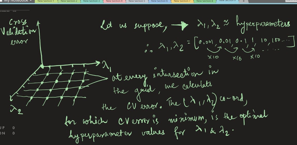
1. Grid Search (Heuristic search/ Brute force / Trial & Error way) — We know that in logistic regression, the regularization hyperparameter lambda (λ) is a real-valued hyperparam. Hence, there are infinite values that lambda can take, and it is impossible to search for all of them. Instead, we take a bunch of logarithmic values starting from 0.001 and multiply 10 with it (a logarithmic search space ensures we are searching a larger space) to get the next value.
After we have our values of lambda for trials, we plot them against the cross-validation errors of the model for each such lambda. Now, the value of lambda for which the cross-validation error is minimum will be the optimal value for lambda hyperparam.
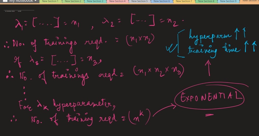
Note: As the number of hyperparameter increases, the number of times, the model needs to be trained for values of that hyperparam, to plot it against the CV errors, also increases exponentially. For machine learning algorithms, we have very few hyperparams to tune, and hence grid search is cool there. But in deep learning, there being tons of hyperparams, grid search will cost lots of training time, hampering model performance. That’s why for bigger set of hyperparams, we use a technique called Random Search.
2. Randomized Search — As the name suggests, in randomized search, unlike grid search, which takes an entire logarithmic search space and plots it against cross-validation errors, we take an interval of logarithmic search space, and every time, a random hyperparam value from that interval is taken to be plotted against the CV error. This is, therefore, greatly helpful in case we have many hyperparams to tune.
Sadly, as the randomized search picks the hyperparameters randomly, it invites a potential risk of missing the ideal hyperparameter values, which may hamper model performance.
3. Bayesian Search — Instead of picking values randomly, why not leverage the Bayes Theorem? Bayesian search is an informed search method, unlike the Grid Search and Random Search, which are heuristic and randomized search, respectively.
Here, using Bayes’ theorem, we calculate the conditional probability of score w.r.t hyperparameters. Hence, if the ‘A’ and ‘B ‘ quantities in Bayes Theorem stand for score and hyperparameter, respectively, Bayes Theorem can be formulated as –
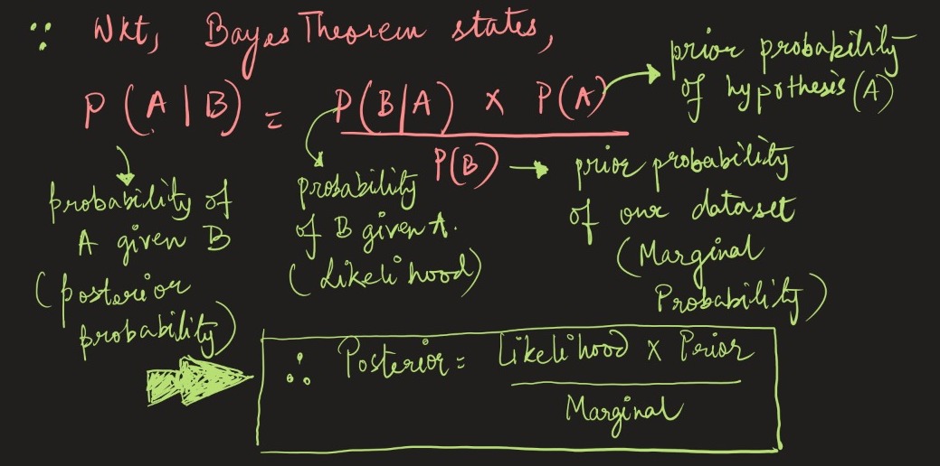
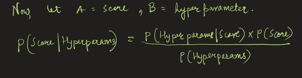
Using Bayes’ Theorem, we perform Bayesian Optimization, where the upcoming hyperparameter to choose is determined based on the prior evaluations. This is why it is called ‘Informed Search’ since the next hyperparams are picked based on previous iterations of the algorithm.
Due to this way of hyperparameter optimization, we neither have to trial and error the entire set of hyperparams nor have to pick random values.
Q5. What is the cross-entropy of loss?
A: Cross Entropy is a powerful loss function to calculate classification prediction error.
A log loss function calculates a probabilistic value for every class. Hence, we can predict the output class based on the likelihood score. This helps to penalize misclassifications, which need to be taken care of to produce a robust classification pipeline.
Let’s see how cross-entropy or multi-class log loss is calculated –
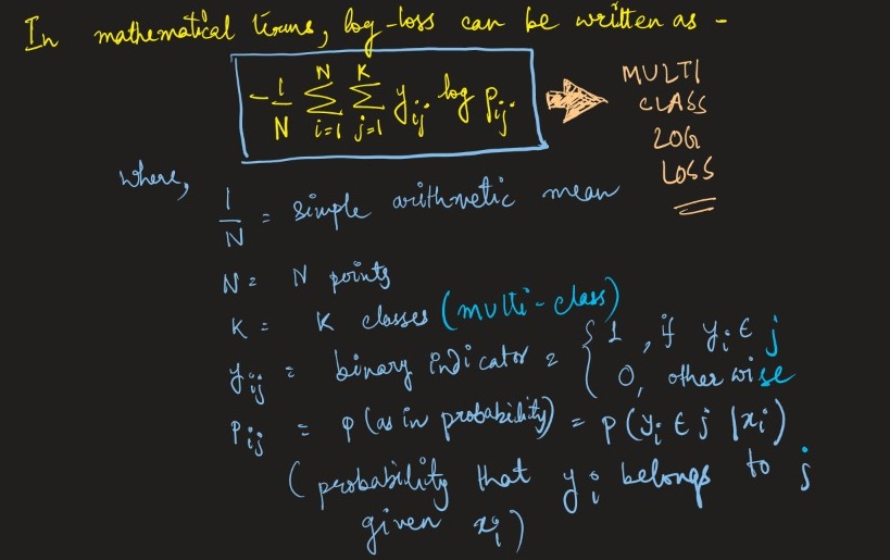
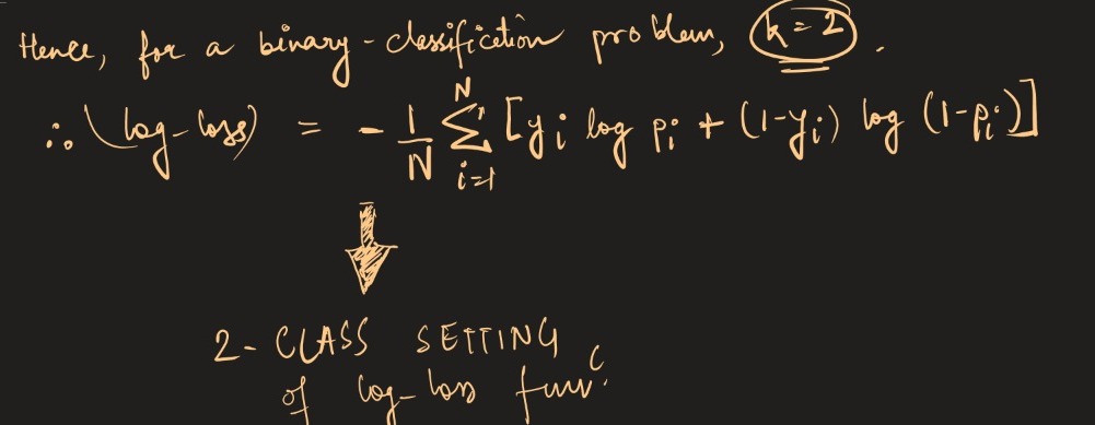
The usage of 1/N in the above image is the concept of entropy (related to thermodynamics), which is the average of the uncertainty of certain information (here, for loss functions, it is the error value). Hence, the name cross-entropy. Generally, we may have K classes if we are doing a multi-class classification. So, for binary or 2-class classification, K = 2. Hence, the cross entropy formula above boils down to –
Q6.What is the goal of A/B testing?
A: A/B testing is an essential and powerful concept used in technology and science to compare two versions of a system/software or any metric and determine which one yields better results or profitability to the organization’s business goal. It is interchangeably called Bucket Testing, Split Testing, or Controlled Experiments.
Imagine you are a machine learning engineer in Amazon’s Alexa team. There is a pre-existing version of Alexa (say, v.1.0). There is a newly released version (say, v.1.1), which the testing team has tested, and every time it yields better results than v.1.0. Now, before rolling out this new version to millions of customers/users, it must be checked whether it is good enough as an upgraded software or not. So, it needs to be sent to production for a set of valuable customers to provide feedback.
To do this, you will select a bunch of trustworthy users who have joined your software’s Beta Program. You will randomly group these users into two groups, A and B. You allocate 90% of your Beta users to group A for feedback on the old model and the rest 10% to group B, for the newly released one. The newly released one is fed to very few users to ensure that a huge amount of customers don’t face any disappointment (if at all).
In this way, they know which version is preferred most by the users and, therefore, whether the end revenue goal is met or not, reducing all sorts of risks.
Q7. When is Ridge regression favorable over Lasso regression?
A: As discussed in Q1 (L1 (Lasso)/ L2(Ridge) regularization methods, we know that –
Ridge Regression forces coefficients/weights towards 0 but never make them equal to 0. This works like enhancing factor for bias term (lambda) and greatly reduces the variance. Thus, this setting in Ridge or L1 regularization helps to fight issues like multicollinearity (where two or more two independent variables/ features are highly correlated). What Ridge does is, it does not remove any feature but keeps all of them, reducing their coefficient values in the model. In this way, we do not lose any contributing features!
On the other hand, Lasso Regression, unlike ridge, readily eliminates the non-contributing features or helps us choose a set of optimal features when we have a lot of them in our data.
Hence, Lasso will risk losing contributing features in cases where many features are correlated to each other and contributing to the prediction. In those multicollinearity cases, we favor Ridge over Lasso, due to its proportional shrinkage rule.
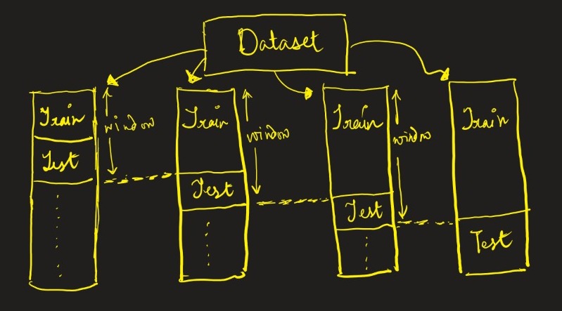
Q8. Can K-fold cross-validation be used on Time Series data? Explain with suitable reasons in support of your answer.
A: K fold cross-validation is a standard and frequently used cross-validation technique, where we split our entire dataset into k (fairly) independent splits or partitions. Then we train exactly (k-1) splits, and the remaining split is used for testing. This process is repeated for every fold, and after each of the folds is tested, the error obtained on each folds is averaged, and the standard deviation is calculated.
In time series data, we cannot use K-fold cross-validation. K fold cross validation is a red flag for time series data because of the high dependency between records/data in time series. In time series, every record is dependent on each other; therefore, the order in time series data needs to be strictly maintained to observe trends. In time series, every record at a particular timestamp is the future record obtained from its previous timestamp record. Using k fold in time series would mean we are peeking upon future data, which is unethical in Machine Learning! I mean, who looks at future predictions to calculate the past?
Hence, we cannot split time series data independently.
To perform cross-validation in a time series data, we need to perform cross-validation using the sliding window technique, which helps us preserve the time series’ dependencies. It is a very simple idea. We train a partition of our dataset, forecast its future predictions, and compute the accuracy of the same. Now, our sliding window will shift towards these forecasted points, which will be included in the next training, and so on. In this way, the dependency is never hampered.
Q9. What is Transfer Learning? Give an example.
A: Transfer Learning is a powerful and popular study in machine learning, where models are pretrained on huge datasets for a specific problem, and then its pretrained knowledge is transferred to perform fine-tuned training to solve a subtask on a new dataset.
For a better understanding, look at the image below-
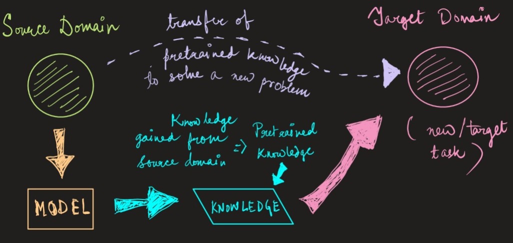
Transfer Learning has become incredibly powerful in recent times due to its awesome generalization, aka domain adaption techniques. The majority of Natural Language and Computer Vision problems are successfully solved using the Transfer Learning approach and perform shockingly better than traditional models which were used earlier in this noble approach.
Example — NLP transfer learning models like BERT, GPT and their variants were pretrained with around~40 GB of crawled text from the internet! This vast knowledge learned by these models, is useful to solve tasks like text summarization, text generation etc. problems without using traditional models and hours or even days of training. Moreover, this approach, used to leverage what’s learned in the source setting to improve generalization in the target setting, produces great robust pipelines.
Q10. What are the data preprocessing techniques to handle outliers? Mention 3 ways that you prefer, with proper explanation.
Outliers are faulty data points found far away from other data points in a dataset. In most cases, they are erroneous and hamper model performance. Hence they should be removed. Outliers are pretty hard to detect, and the following approaches were developed which are useful while detecting outliers –
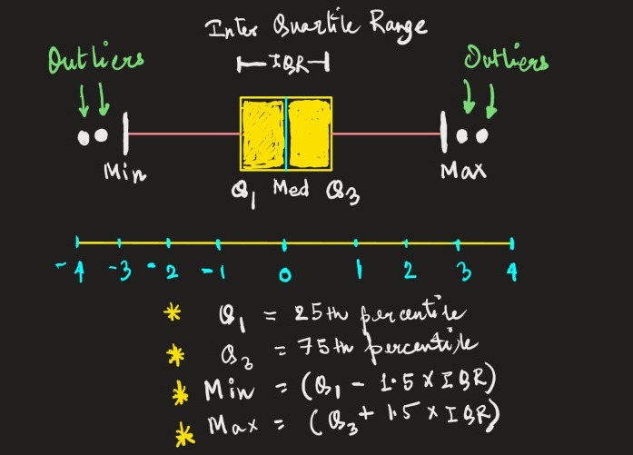
1. Box Plots — Box Plots are a great data visualization tool for detecting outliers. Data scientists extensively use this approach to detect outliers during univariate data analysis. Box plots show the distribution of the dataset using quartiles. It uses the min, first quartile, median, third quartile, and a max of the data. It has kind of line-like bristles protruding out of the box (also called whiskers), showing the variability of data beyond the upper and lower quartiles. The outliers are the dots in box plots, so spotting them becomes very easy.
Now let us see how it looks for a better understanding –
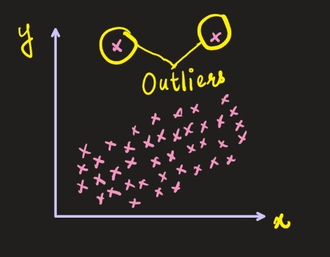
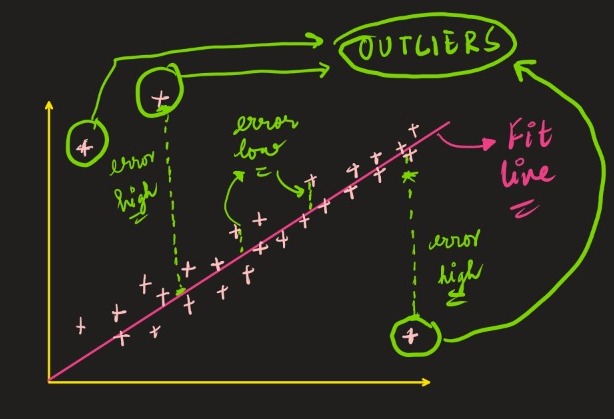
2. Multivariate Analysis — Another good method to detect outliers is a multivariate analysis (like robust regression techniques), where we fit our data with a model and try to find the residual error. Any error value that is a discrepancy (higher than the usual error value) is supposed to be an outlier. Then, we can easily remove those data points.
Let us see how it’s done –
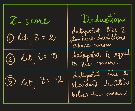
3. Z- Score — In plain English, the Z score is a statistical metric that tells us how distant is a particular record from the rest of the datapoints in the dataset. By definition, the Z score is computed as the total number of standard deviations by which the value of a record is above or below the mean that each value lies at.
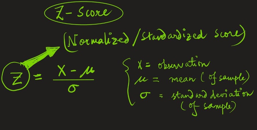
Z score makes use of this concept to detect outliers. The further away an observation’s Z-score is from zero, the more outlier-ish it is. A generally preferred cut-off for z-score is (3,-3).
Q11. Mention one disadvantage of Stochastic Gradient Descent.
A: One of the major drawbacks of Stochastic Gradient descent is that it is computationally much more expensive compared to gradient descent and mini-batch gradient descent due to very frequent weight updates and exploiting all resources during every training. Also, frequent weight updates create too much noise towards its path to the global minima. Hence, convergence is too noisy, which may create a deflecting path from the minima to other directions.
Q12. What is the purpose of a ROC curve?
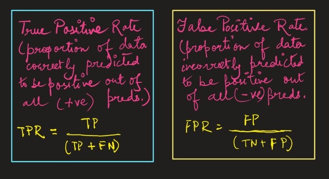
A: ROC Curve plots the True Positive Rate (TPR) against the False Positive rate (FPR) to help visualize the performance of a classification task ( more preferred in binary classification).
Interpretation –
A ROC that outputs curves closer to the top-left corner of the graph indicates the good performance of the classifier used. If the curve comes closer to the 45-degree diagonal area of the ROC space, it indicates the poor performance of the classifier used.
Q13. Why is a validation set necessary?
A: A validation set is a part of our dataset that is used after training a model to check how it performs on unseen data. Based on the accuracy and evaluation of the model’s performance on the validation set, the information can be further used to perform hyperparameter optimization to yield better performance or to figure out if the model is overfitting or underfitting. Hence, a validation set is very useful for any Machine Learning pipeline for generalization and robustness of the pipeline.
Q14. When is one hot encoding favored over label encoding?
A: One hot encoding is a standard natural language processing technique that converts (or, encodes) categorical variables into binary vectors for the machine to learn patterns to text (categorical variables, like ‘yes’, and ‘no’). Whereas label encoding converts categorical variables into numerical values.
Though both techniques work almost similarly, machine learning algorithms often incorrectly interpret the numerical values produced by label encoding. Numerical values tend to impose some order or relationship between them, which the machine learning model tends to take seriously, yielding abnormal/wrong predictions. Due to this reason, binary encoding (one hot encoding) is favored more nowadays over label encoding.
Q15. What is the curse of dimensionality? Why do we need to reduce it?
A: Let us first see a very crisp and understandable definition of the Curse of Dimensionality –
A phenomenon that occurs when the dimensionality of the data increases, the sparsity of the data increases.
While solving any Machine Learning problem, we visualize our data and learn more about it before getting to the modeling part. Data Cleaning, Preprocessing, and Feature Engineering needs to be taken very seriously before applying any ML model to the data. One of the major challenges faced while solving an ML problem at hand is the increasingly high number of features (aka high dimensions) that real-world datasets tend to have. It means we may have thousands of features to take for training. Imagine the computational cost!! Huge.
The curse of Dimensionality is really a CURSE. It makes training extremely slow-paced, hampers model performance, and often introduces overfitting due to overlearning or fitting too close to the training data. It fails to predict the test/ unseen data well.
To address this issue, we need to reduce the dimensions of our data. Or in Machine Learning terms, we need to exclude unnecessary features from modeling without losing valuable information. This will help us to speed up the training process, model it better, and arrive at an optimal solution.
Tips for your Machine Learning Interview
To ace your Machine Learning interview, you must take care of the below tips –
1. Prepare all the foundational concepts of Statistics and Probability, Linear Algebra that is used in the basic Machine Learning algorithms. Make sure you are well-equipped with all the traditional ML algorithms and techniques and have an idea of how they work under the hood.
2. Have a product sense of the company where you will be interviewed. (the kind of analytics they do, the kind of data and business problems they work on)
3. Practice implementing ML techniques/algorithms before the interview. Spend at least 2 hours a day studying Kaggle’s top-voted notebooks by searching topics with a simple keyword. Read Scikit Learn Documentations of various algorithms and approaches. They are very professionally designed and helpful.
4. Pick problem statements from various Kaggle competitions and try to solve them (remember, it is perfectly fine to view what others did and take ideas, but make sure you code your notebook all by yourself!). Try to pick up real-world problems, and avoid toy problems like Diabetes Prediction or House Price Prediction. Get out of the beginner zone as fast as you can.
5. Brush up your SQL and Python coding skills. Without SQL, there is no way to get through a DS/ML interview.
6. Study your resume properly. Try to explain what challenges you faced in the projects you did, and how you solved them, rather than just giving a vague explanation.
and lastly,
7. Stay true to yourself, and do not try to make up answers to things you don’t know. Just humbly say you really don’t know the answer to that, but you surely will work on it! HELPS A LOT!
Conclusion
Cheers on reaching the end of this article! Hope this article will help you ace your data science interviews.
Your key takeaways from this article are-
1. You learned in-depth about very important Machine Learning fundamentals and advanced topics like Hyperparameter Optimization, Transfer Learning, Dropouts, Regularization, etc. The topics discussed here are very important and are very, very common in any small to big organization’s ML interview.
2. Tips on acing your upcoming machine learning interview.
All the best!🙌🏼
The media shown in this article is not owned by Analytics Vidhya and is used at the Author’s discretion.
An ace multi-skilled programmer whose major area of work and interest lies in Software Development, Data Science, and Machine Learning. A proactive and detail-oriented individual who loves data storytelling, and is curious and passionate to solve complex value-oriented business problems with Data Science and Machine Learning to deliver robust machine learning pipelines that ensure maximum impact.
In my free time, I focus on creating Data Science and AI/ML content, providing 1:1 mentorships, career guidance and interview preparation tips, with a sole focus on teaching complex topics the easier way, to help people make a successful career transition to Data Science with the right skillset!


