High Accuracy Lightweight and Superfast Model Nanodet Plus

This article was published as a part of the Data Science Blogathon.

Introduction

NonoDet – Plus is a Super fast, highly accurate – lightweight, and anchor-free object detection model, and it’s working in real-time on mobile devices. Before getting into knowing about Nanodet, we should know about FCOS (Fully Convolutional One-Stage Object Detection). Since the invention of convolutional neural networks, anchor-based approaches like FasterRCNN, RetinaNet, and SSD have dominated the field of object detection. These techniques rely on many pre-set anchors that are tiled over the image. Each anchor forecasts the refinement of the coordinates and if an object is confined.

FCOS (Fully Convolutional One-Stage Object Detection)

More focus has recently been placed on removing the need for preset anchors, which necessitate manual alteration of the scale, aspect ratio, and several anchors. To do that, FCOS, and efficient approach that directly finds objects based on dots tiled on the image, was presented.

This model was well-liked because it could match the performance of anchor-based techniques while requiring fewer predictions per image.

Forward Pass

A pyramid-shaped FCOS is constructed on top of FPN, with multi-level aggregating features from the backbone. Five feature levels of predictions are collected from FPN.
Following that, a subnetwork with three branches 1. classification, 2. centredness, 3. regression—is fed the outputs.
Here, we’ll talk about the forward pass pipeline.

Input: A image that is [B, H, W, 3] in size.

BackBone: To be FPN-compatible, multi-scale properties are removed from a CNN encoder. Any recently in-use encoder, such as DenseNet or ResNet, can be attached to deliver as the feature extractor. For ResNet50, we use the final feature maps from stages 1 through 5.

C1: [B, H/2, W/2, 64]    
C2: [B, H/4, W/4, 256] 
C3: [B, H/8, W/8, 512]  
C4: [B, H/16, W/16, 1024]
C5: [B, H/32, W/32, 2048]

FPN 

FPN utilises the scale-invariant characteristics of feature pyramids. As a result, the model can detect things at many scales. While shallow layers have a great resolution but few semantic features, deeper layer features encode lower resolution but richer semantic information. Lateral integrations are used to combine features between the shallow and deeper layers of the pyramid to balance both effects. This improves the precision of finding and locating objects of many sizes. Microscopic objects are improved.

With an output channel of 256, each feature map is scaled by a factor of two. The output stride is typically used to describe the scale or ratio of the output feature to the input image.

P3: [B, H/8, W/8, 256]    
P4: [B, H/16, W/16, 256] 
P5: [B, H/32, W/32, 256]  
P6: [B, H/64, W/64, 256]
P7: [B, H/128, W/128, 256]

Detection Head Per Pixel Predictions 

FCOS produces the predictions in the same way for all layers spanning FPN, analogous to fully convolutional segmentation CNNs, where each pixel in the output layer corresponds to a confidence score of the semantic scores.

Shared Head Branches: Three heads are used to estimate the per-pixel prediction, and each head branch uses a full convolution network (FCN) with the same architecture as that shown below.

head = [[Conv2d, GroupNormalization, relu],
        [Conv2d, GroupNormalization, relu],
        [Conv2d, GroupNormalization, relu],
        [Conv2d, GroupNormalization, relu]]

Note that all FPN features share the same head. i.e., the same head is used to feed each level in FPN.

Centre-ness Head

The centre-ness distinguishes between an object’s position and its centre. After observing that scores for low-quality boxes distant from the centre remained high, the authors suggested including this. Therefore, they can be suppressed by learning this centeredness scale component.
For each feature level, it is responsible for the centre-ness head will output the normalised distance from the object’s centre. The forecast is closer to the centre, the higher the normalised value.

P3_ctrness: sigmoid(head(P3))   # [B, H/8, W/8, 1]  
P4_ctrness: sigmoid(head(P4))   # [B, H/16, W/16, 1]
P5_ctrness: sigmoid(head(P5))   # [B, H/32, W/32, 1] 
P6_ctrness: sigmoid(head(P6))   # [B, H/64, W/64, 1] 
P7_ctrness: sigmoid(head(P7))   # [B, H/128, W/128, 1]

Class Predictions Head 

Forecasts the per-pixel class probability with the centre-ness score as the weighting factor. As mentioned above, the class probability is calculated by multiplying the class probability by the centre-ness score.

P3_class_prob: sigmoid(head(P3)) * p3_ctrness # [B, H/8, W/8, C]  
P4_class_prob: sigmoid(head(P4)) * p4_ctrness # [B, H/16, W/16, C]
P5_class_prob: sigmoid(head(P5)) * p5_ctrness # [B, H/32, W/32, C]
P6_class_prob: sigmoid(head(P6)) * p6_ctrness # [B, H/64, W/64, C]
P7_class_prob: sigmoid(head(P7)) * p7_ctrness # [B, H/128, W/128, C]

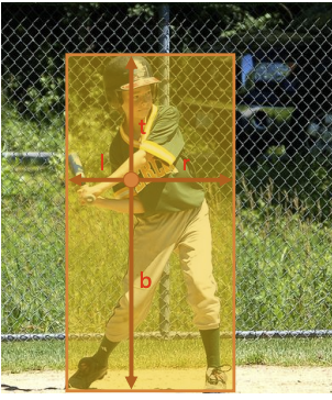
Box Regression Head

 Predicts the (l, t, r, and b) from the location’s centre.

P3_reg: conv2d(head(P3))   # [B, H/8, W/8, 4]  
P4_reg: conv2d(head(P4))   # [B, H/16, W/16, 4]
P5_reg: conv2d(head(P5))   # [B, H/32, W/32, 4] 
P6_reg: conv2d(head(P6))   # [B, H/64, W/64, 4] 
P7_reg: conv2d(head(P7))   # [B, H/128, W/128, 4]

The regression head has been trained to forecast scale normalised distances, it should be noted. Therefore, we must denormalise to picture size during inference reg = reg pred * stride. The next section will describe how to map pixel predictions to a location.

NanoDet

The final Nanodet-Plus trained model will be less than 1.8 MB in size, highly lightweight, and extremely fast—97 frames per second on a mobile ARM CPU. Nanodet Plus offers high precision: It has much lower memory costs than other models, has up to 34.3 mAP, and is a training-friendly model that employs a GPU. The batch-size=80 option is accessible on a GTX1060 6G. It is simple to set up because it supports several backends, including ncnn, MNN, and OpenVINO. Provide an Android demonstration that uses the NCNN inference framework as well.
Generalized Focal Loss is used for regression loss and classification in NanoDet, a one-stage, anchor-free item detection model in the FCOS approach.
In NanoDet-Plus, we present a novel label assignment technique that employs a basic assign guidance module (AGM) and a dynamic soft label assigner to handle the optimal label assignment problem in lightweight model training (DSLA). The Ghost-PAN light feature pyramid, which improves multi-layer feature fusion, is also available. These improvements increase the detection accuracy of previous NanoDet on the COCO dataset by 7 mAP.

Nanodet Custom Dataset Training

Conclusion

Given its ease of use while being on par with anchor-based techniques, NanoDet – FCOS is undoubtedly a positive development in the field of object identification research. I’m excited to see what happens next development and growth in this field.

The key lessons from the aforementioned FCOS and Nanodet are summarized as follows:

• We gained knowledge of FCOS and its Components of FCOS.
• We take in the fundamentals of Nanodet.
• We gained knowledge about how to train Nanodet Custom Dataset Training.

Reference: https://github.com/RangiLyu/nanodet

The media shown in this article is not owned by Analytics Vidhya and is used at the Author’s discretion.

Parthiban Marimuthu

I'm Parthiban and I have more than one year experience in Machine Learning and Deep Learning. A Mechanical Engineering enthusiast with the passion to learn more about Machine Learning and emerging technology in the world. Study and transform data science prototypes and Design machine learning systems. Research and implement appropriate ML algorithms and tools. Develop machine learning applications and select appropriate datasets and data representation methods. Perform statistical analysis and fine-tuning using test results, and extend existing ML libraries and frameworks.