A Guide on Social Network Recommendation System

This article was published as a part of the Data Science Blogathon.

Introduction

The recommender system foresees users’ preferences and generates recommendations or proposals based on those preferences. Well-known websites like Facebook, LinkedIn, Instagram, Snapchat, Twitter, Amazon, Flipkart, and Netflix use different machine learning algorithms to draw people and increase their time spent on their websites and services.

• Social Network Service Recommendation System
• Streaming Service Recommendation System
• Tourism Service Recommendation System
• E-Commerce Service Recommendation System
• Healthcare Service Recommendation System
• Education Service Recommendation System

Every recommendation engine uses a different approach. We’ll mostly be talking about Social Network Service recommendations in this article.

What is Recommendation System?

The Social Network Service Recommendation System uses several algorithms to suggest many people possible who may end up becoming friends with the user. The Link Prediction Method is undoubtedly a common type of algorithm for recommendations. Let’s talk about how recommendations are made by applying the Link Prediction Method.

Link Prediction Method

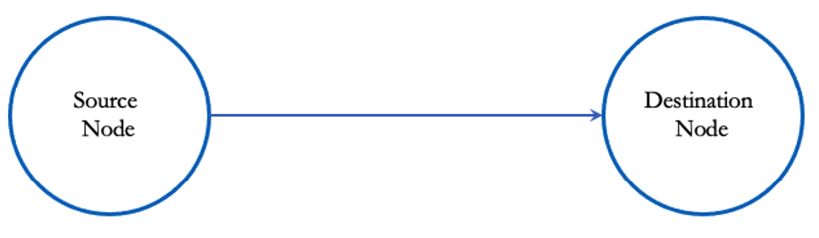
In Link Prediction Method, every single user is a node. Edges represent the relationship between two nodes. We can say that two nodes are related if there exists a relationship between them. As nodes and links can be represented in graphs, graph theory concepts can be used to make link predictions. Both directed and undirected graphs are possible. Because nodes in social networks can have followers and followings, the graph looks directed.

The link Prediction method should identify all probable connections from the source node to other nodes.

Approach

The model should be trained using the given set of nodes together with their corresponding independent features. The model should predict all potential links to establish a connection if a new source node is made available. If a link can be established, recommendations from friends can be sent from the source node to the destination node.

We used the dataset from the Facebook Recruiting competition on Kaggle to train our model.

Dataset

There is a training dataset and a testing dataset for the Facebook Recruiting competition on Kaggle. The training set has 9437519 rows and two columns (source node, destination node). The test set has 262588 rows and 1 column (source node). Here is a link to the dataset.

Task

To find all functional connecting nodes (destination nodes) for the given source nodes in the test dataset.

Challenges

When we look into the dataset, we only find two columns (source node, and destination node). There is no target variable. We are unable to develop a machine-learning model using these features. More features must be added. Noisy data may occur when the number of features rises. Our difficulty is to,

• Make a target variable
• Including features (Feature Engineering)
• Eliminating irrelevant features (Feature Selection)

Let’s build our recommendation engine piece by piece.

Steps to Perform the Recommendation System

1. Importing necessary libraries
2. Exploratory Data Analysis
3. Creating Missed Connections
4. Getting train and test data after concatenation
5. Feature Engineering
6. Feature Selection
7. Model Training
8. Hyperparameter Tuning
9. Performance Measure

Importing Libraries

Let’s load the necessary libraries, including Seaborn, Pandas, NumPy,
Matplotlib, and SKLearn.

Exploratory Data Analysis

Based on the dataset, we can draw certain conclusions.

 1. A Directional Graph

import pandas as pd
train_df = pd.read_csv('train.csv')
print(train_df.head(10))
print(train_df.shape)

The source node 1 is linked to the destination nodes 690569, 315892, and 189226, according to the above table. We may say that the above graph is a directed graph because the link between the source and destination nodes is visible.

2. Number of unique nodes and links

The number of unique nodes and links is calculated.

g=nx.read_edgelist('train_unique.csv',delimiter=',',create_using=nx.DiGraph(),nodetype=int)
print(nx.info(g))

3. Number of followers(in_degree) & Following/Followee (out_degree)

The functions in_degree() and out_degree() are used to calculate the total number of followers and followers for each person.

• Follower (in_degree) :
  •  For the Destination node, the Source node is the follower.
•     Following/Followee(out_degree):
  • For the source node, the Destination node is the followee/following

“indegree_no” gives the number of followers of each node.

indegree_no = dict(g.in_degree()).values()

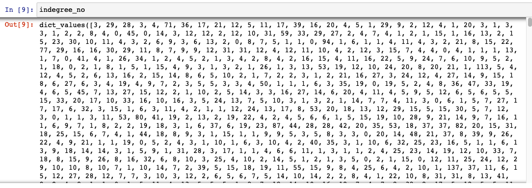
Indegree values

“outdegree_no” gives the
number of followee/following of each node. 

outdegree_no = dict(g.out_degree()).values()

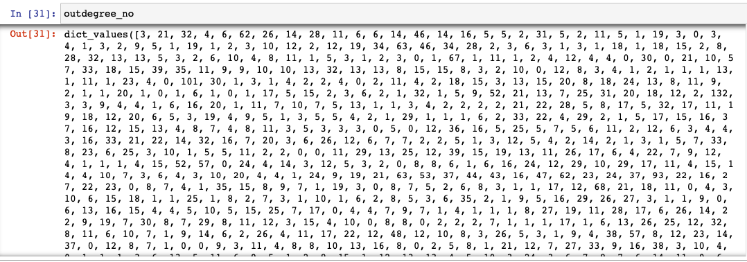
Outdegree values

“in_out_degree” gives the total number of followers + following of each node.

from collections import Counter
dict_in = dict(g.in_degree())
dict_out = dict(g.out_degree())
total = Counter(dict_in) + Counter(dict_out)
in_out_degree = np.array(list(total.values()))

4. The graph’s findings are:

• 14% of participants follow no one.
• 10% of people have no followers at all.
• 10% of people are more popular and have more followers.
• A very small number, 1% of users, have more than 40 followers.
• One percent of users—a relatively small percentage—have more than 72 followers.
• No. of people with a minimum following and followers: 334291
• No. of people with a maximum following and followers: 1
• No. of people with less than 10 following and followers: 1320326
• Components that lack a path between them: 32195

Creating Missed Connections

To formulate the target variable, we should create new edges called missed edged with the aid of exploratory data analysis. The following is our understanding:

• We need data on linked and disconnected nodes (0 and 1) for the categorization problem.
• Until now, we have only been given the details of neighboring nodes.
• We should add details about the disconnected nodes.
• The maximum number of links established with ‘n’ nodes: nC₂
• There are possibilities for 1862220 nodes to generate1862220C2 links, in which 9437519 are neighbors and are denoted by 1.
• The remaining nodes can be represented by 0 and are unconnected.
• The maximum number of
  possible not-connected nodes is 1862220C₂-9437519.
• The nodes with the shortest paths longer than two are our current focus.
  • The value of the disconnected nodes must always be zero because there is no connection.
  • Add a 0 to the new connection.

How to fill in missing edges:

1. Read unique valued train dataset.
2. Make a dictionary to store (1 or -1) as a value and (source node, destination node)
   as a key.

• ‘1’ represents that the source and destination are neighbors
• ‘-1’ represents that the source and destination aren’t related
• Look for nodes in the training set and mark them as ‘1’.
• Create an empty set to add not-connected links.
• Create source and destination nodes randomly, with a size of 1862220 each, and initialize them with -1 to signify that they have no relationship.
  • The reason to choose 1862220 source and destination nodes is, that they have the potential to produce 9437519 links.
• Consider the following to complete the set of missing edges:
  • Edges shouldn’t have been joined before.
  • The source node and the destination node shouldn’t be the same.
  • The shortest path between nodes is > 2
    

    ###generating disconnected edges from given graph
    import random
    if not os.path.isfile('missing_edges_final.p'):
        #getting all set of edges
        r = csv.reader(open('train_unique.csv','r'))
    #     r = pd.read_csv('train_unique.csv')
        edges = dict()
        for edge in r:
            edges[(edge[0], edge[1])] = 1  # marking edges present as 1
        missing_edges = set([])
        while (len(missing_edges)<9437519):
            a=random.randint(1, 1862220)
            b=random.randint(1, 1862220)
            temp = edges.get((a,b),-1)   # marking random edges as -1
            if temp == -1 and a!=b:
                try:
                    if nx.shortest_path_length(g,source=a,target=b) > 2: 
                        missing_edges.add((a,b))
                    else:
                        continue  
                except:  
                        missing_edges.add((a,b))              
            else:
                continue
        pickle.dump(missing_edges,open('missing_edges_final.p','wb'))
    else:
        missing_edges = pickle.load(open('missing_edges_final.p','rb'))

    
    

     

    
    
• Checking both datasets
  has an equal number of links.

    df_pos = pd.read_csv('train.csv')
    df_neg = pd.DataFrame(list(missing_edges), columns=['source_node', 'destination_node'])
    print("Number of nodes in the graph with edges", df_pos.shape[0])
    print("Number of nodes in the graph without edges", df_neg.shape[0])

• Concatenate the positive
  and negative datasets into one dataset after equating the two datasets.

The Shortest path

The intuition of the shortest path is:

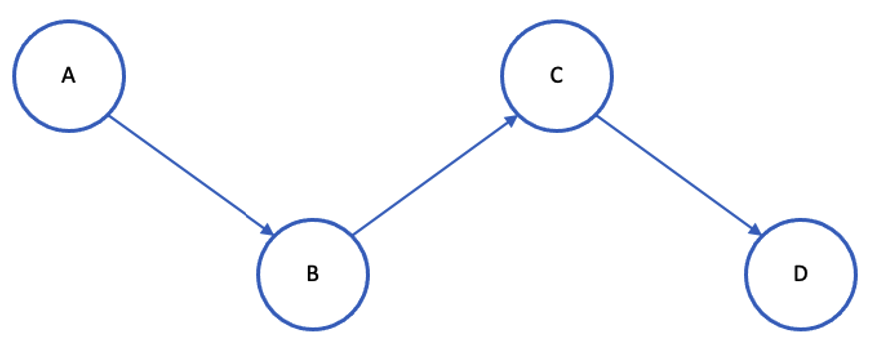
Finding the shortest route between a source and a destination is made easier by using the shortest path.

If A is the source and D is the destination in the image above, the shortest path between

• A – B = 1
• A – C = 2
• A – D = 3

Compared to linking nodes A and D, connecting nodes A and C has a higher likelihood. The desired value should be 0; thus, to generate disconnected nodes, we employ pairs that could not be joined in the future. The nodes whose shortest paths above two are only considered.

Getting Trained and Test Data after Concatenating Linked and Missed Nodes

The formation of target variables is complete. The dataset should now be divided into training and testing sets. By dividing the dataset, we can do a performance analysis.

• Split train and test datasets from the concatenated dataset
• Verify that the training dataset contains every node that was present in
  the test dataset.

    trY_teY = len(train_nodes_pos.intersection(test_nodes_pos))
    trY_teN = len(train_nodes_pos - test_nodes_pos)
    teY_trN = len(test_nodes_pos - train_nodes_pos)
    print('no of people common in train and test -- ',trY_teY)
    print('no of people present in train but not present in test -- ',trY_teN)
    print('no of people present in test but not present in train -- ',teY_trN)
    print(' % of people not there in Train but exist in Test in total Test data are {} %'.format(teY_trN/len(test_nodes_pos)*100))

Important learning made from the result of the above code is,

The percentage of nodes present in the test dataset but absent from the training dataset is 7.12%. We lack the knowledge necessary to make recommendations for these nodes. This leads to a partial cold start problem. We are employing the Representative-Based Approach to lessen this.

Use a sample of the data from both datasets to train the model. We randomly picked 50,000 data from the test dataset and 100,000 data from the training dataset.

    filename = "train_after_eda.csv"
    n_train = sum(1 for line in open(filename)) 
    n_train =  15100028
    s = 100000 #desired sample size
    skip_train = sorted(random.sample(range(1,n_train+1),n_train-s))

Feature Engineering

We have only the source node and the destination node right now. To train a model, these two features are insufficient. We would like to add more features. Utilizing the relationship between the nodes, we will create more features.

Jaccard Distance:

The likelihood of a link between the source node and the destination node is measured by the Jaccard distance. We can calculate this distance for both followers and following.

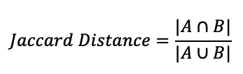
Let A be a set of followers of the source node

Let B be a set of followers of the destination node

A = {1,5,7,9,11,13}, B = {3,11,13,15,17,19}

A ∩ B = {11, 13}, |A ∩ B| = 2

A ∪ B = {1,3,5,7,9,11,13,15,17,19} , |A ∪ B| = 10

Jaccard Distance = 2/10

The probability of connection between A and B is 0.2

 

The likelihood of a connection between source and destination nodes is 0.2 and grows with the number of common nodes. A connection between nodes is more probable if the Jaccard distance is high.

#for followee/following
def jaccard_for_following(a,b):
    try:
        if len(set(train_graph.successors(a))) == 0  | len(set(train_graph.successors(b))) == 0:
            return 0
        sim = (len(set(train_graph.successors(a)).intersection(set(train_graph.successors(b)))))/
                                    (len(set(train_graph.successors(a)).union(set(train_graph.successors(b)))))
    except:
        return 0
    return sim

Cosine Similarity:

The similarity between two links is quantified by cosine similarity. It’s represented by the cosine angle between them. The likelihood of a connection is higher if the cosine angle between the source and destination is zero or close to zero.

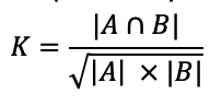
For the above example, cosine similarity for followees/following can be calculated as:

|A ∩ B| = 2

|A| = 6

|B| = 6

K = 2 / √36 ; K = 0.667

 

#for followees
def cosine_for_following(a,b):
    try:
        if len(set(train_graph.successors(a))) == 0  | len(set(train_graph.successors(b))) == 0:
            return 0
        sim = (len(set(train_graph.successors(a)).intersection(set(train_graph.successors(b)))))/
                                    (math.sqrt(len(set(train_graph.successors(a)))*len((set(train_graph.successors(b))))))
        return sim
    except:
        return 0

Page Rank:

Page Rank is determined by two factors: the number of links and the quality of links.

• The number of links
  • It counts the number of incoming links (followers)
• Quality of links
  • It considers the incoming links (followers) that already have more incoming links (followers).

pr = nx.pagerank(train_graph, alpha=0.85)

Shortest Path:

Based on the weights, the shortest path will determine the shortest route from the source node to the destination. If there exists a direct link between the source and the destination node, we will delete that link. This direct link won’t contribute much to prediction.

#if has direct edge then deleting that edge and calculating shortest path
def compute_shortest_path_length(a,b):
    p=-1
    try:
        if train_graph.has_edge(a,b):
            train_graph.remove_edge(a,b)
            p= nx.shortest_path_length(train_graph,source=a,target=b)
            train_graph.add_edge(a,b)
        else:
            p= nx.shortest_path_length(train_graph,source=a,target=b)
        return p
    except:
        return -1

Weakly Connected Component:

Here neither the source nor the destination can be reached from the other.

wcc=list(nx.weakly_connected_components(train_graph))
wcc gives a list of weakly connected components.

• We need to check if the source and destination nodes are part of the wcc.
• If they are both present
  in wcc, remove that link and find the shortest path.
• If both the nodes are in wcc, assign 1.
• If one of the nodes is not in wcc, assign 0.

#getting weekly connected edges from graph 
wcc=list(nx.weakly_connected_components(train_graph))
def belongs_to_same_wcc(a,b):
    index = []
    if train_graph.has_edge(b,a):
        return 1
    if train_graph.has_edge(a,b):
            for i in wcc:
                if a in i:
                    index= i
                    break
            if (b in index):
                train_graph.remove_edge(a,b)
                if compute_shortest_path_length(a,b)==-1:
                    train_graph.add_edge(a,b)
                    return 0
                else:
                    train_graph.add_edge(a,b)
                    return 1
            else:
                return 0
    else:
            for i in wcc:
                if a in i:
                    index= i
                    break
            if(b in index):
                return 1
            else:
                return 0

Adar Index:

The Adar Index calculates the number of common links that two nodes share.

It uses the formula:

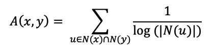
Whereas,

N(x) = Followers and following of x
N(y) = Followers and following of y

Let

N(x) = {e1,e3,e5,e7}
N(y) = {e1, e3,e7,e9,e11}

N(x)∩N(y) = { e1,e3,e7}

For every edge of N(x)∩N(y), we should take the inverse log and sum them.

N(x)∩N(y) will give two types of insights.

Celebrity Link

Since both follow celebrities, there will be some common links between the source and destination nodes. It does not necessarily follow that both nodes are friends. The inverse log decreases the Adar index value and hence lowers the likelihood of a friend recommendation.

Normal Link:

There may be a potential for both nodes to be friends given the small number of common links between the source and destination nodes. The Adar index’s value rises after applying inverse log, thereby increasing the likelihood of being a friend and will recommend you.

#adar index
def calc_adar_in(a,b):
    sum=0
    try:
        n=list(set(train_graph.successors(a)).intersection(set(train_graph.successors(b))))
        if len(n)!=0:
            for i in n:
                sum=sum+(1/np.log10(len(list(train_graph.predecessors(i)))))
            return sum
        else:
            return 0
    except:
        return 0

Follow Back:

It’s been believed that if there is a connection between the source and the destination, there exists a connection between the destination and the source. If such a connection exists, assign 1, and if not, 0.

If
train_graph.has_edge (b, a), then return 1; otherwise, return 0.

def follows_back(a,b):
    if train_graph.has_edge(b,a):
        return 1
    else:
        return 0

Katz Centrality:

It calculates the relative influence by counting the number of neighbors and those who are linked to the node. It is employed to assess a node’s relative power among the nodes.

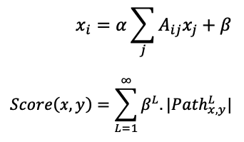
Where,

    katz = nx.katz.katz_centrality(train_graph,alpha=0.005,beta=1)

HITS(Hyperlink-Induced Topic Search) Score:

• They go by the names hubs or authority.
• Using the HITS score we can extract authority and hub value.
• It is based on a webpage rating.
  • Authorities: The node values that are supported by many other hubs
  • Hubs: The node value supported on outgoing links

    hits = nx.hits(train_graph, max_iter=100, tol=1e-08, nstart=None, normalized=True)

Weight Features:

Edge weight is necessary to assess the similarity between nodes. The weight lowers when the number of links increases, and vice versa.

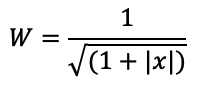
for i in  tqdm(train_graph.nodes()):
    s1=set(train_graph.predecessors(i))
    w_in = 1.0/(np.sqrt(1+len(s1)))
    Weight_in[i]=w_in
    s2=set(train_graph.successors(i))
    w_out = 1.0/(np.sqrt(1+len(s2)))
    Weight_out[i]=w_out

Preferential Attachment:

In social networks, people who have more friends are more inclined to continue adding friends to their side. By dividing the number of friends a node has, we may determine how rich it is. Both the following and the followers will benefit from this.

def Preferential_Att1_Followers(x,y):
    try:
        if len(set(train_graph.successors(x)))==0|len(set(train_graph.successors(y)))==0:
            return 0
        score=(len(set(train_graph.successors(x)))*len(set(train_graph.successors(y))))
        return score
    except:
        return 0

Feature Selection

We have added many new features through feature engineering. Some may be unimportant or noisy, making the machine learning model perform worse. During the deployment, adding new features will make the algorithm more difficult. Maintaining features that provide the best performance is crucial. Techniques for feature selection assist us in doing so. Here, the feature selection is made using the Recursive Feature Elimination with Cross Validation.

Recursive Feature Elimination with Cross Validation:

Working Steps:

• Constructs a model with all the features.
• Deletes features with less importance.
• Rebuilds the model with the remaining features.
• Repeat this until no more features can be discarded.

Why RFECV:

• Reduces model complexity
• Easy to configure and use
• Collinear and linearly dependent features are removed automatically.
• Returns the optimal number of features for the model
• Captures all features important for model training

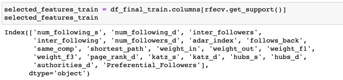
Here, the REFCV algorithm returned 20 important features.

from sklearn.feature_selection import RFECV
rfecv = RFECV(estimator= XGBClassifier(random_state=25,n_jobs=-1), cv = 5)
rfecv.fit( df_final_train,y_train)
X1_cv = rfecv.transform( df_final_train )
X2_cv = rfecv.transform( df_final_test)
f = rfecv.get_support(1)
f

Model Training

Our model needs to be trained now. Our model was trained using 4 different machine learning algorithms.

• XGBoostClassifier
• RandomForestClassifier
• KNearestNeighbor
• SupportVectorMachine

Hyperparameter Tuning the Recommendation System

To identify the best parameters, we performed hyperparameter tuning. The results are tracked.

XGBoostClassifier:

The following parameters were used to evaluate the performance of the XGBoostClassifier Algorithm.

param_dist = {"n_estimators":sp_randint(105,125),
              "max_depth": sp_randint(1,10),
              "alpha": [0.001,0.01,0.1],
              "learning_rate":[0.001,0.01,0.1]}
clf = XGBClassifier(random_state=25,n_jobs=-1)
rf_random = RandomizedSearchCV(clf, param_distributions=param_dist,
                                   n_iter=5,cv=10,scoring='f1',random_state=25,return_train_score=True)
rf_random.fit(X1_cv,y_train)

Random Forest classifier:

Using the following parameters, the RandomForestClassifier Algorithm’s performance was assessed.

param_dist = {"n_estimators":sp_randint(105,125),
              "max_depth": sp_randint(10,15),
              "min_samples_split": sp_randint(110,190),
              "min_samples_leaf": sp_randint(25,65)}

rf_clf = RandomForestClassifier(random_state=25,n_jobs=-1)
rf_random = RandomizedSearchCV(rf_clf, param_distributions=param_dist,
                                   n_iter=5,cv=10,scoring='f1',random_state=25,return_train_score=True)
rf_random.fit(df_final_train,y_train)

KNearest Neighbor:

Using the following parameters, the KNearestNeighbor Algorithm was analyzed for improved performance.

param_dist = {"n_neighbors":sp_randint(5,10)}
k_clf = KNeighborsClassifier(n_jobs=-1)
rf_random = RandomizedSearchCV(k_clf, param_distributions=param_dist,
                                   n_iter=5,cv=10,scoring='f1',random_state=25,return_train_score=True)
rf_random.fit(df_final_train,y_train)

Support Vector Machines:

param_dist = {"alpha": sp_randint(1,3)}
svm_clf = SGDClassifier(n_jobs=-1)
rf_random = RandomizedSearchCV(svm_clf, param_distributions=param_dist,
                                   n_iter=5,cv=10,scoring='f1',random_state=25,return_train_score=True)
df_final_train=df_final_train.astype(float)
rf_random.fit(df_final_train,y_train)

Performance Measure of Recommendation System

The most important part of the recommendation system is the overall performance metric. We’ve used a variety of models to get performance scores. Choose the one that works for you.

We have computed the f1 score before and following the feature selection, and the values are given below.

Conclusion

Through this article, we’ve gained knowledge about

• Performing Exploratory Data Analysis
• Techniques to seek out missing edges (to create new friend suggestions)
• Feature Engineering
• Feature Selection
• Hyperparameter tuning
• Performance Analysis

This recommendation system heavily relies on feature engineering and feature selection. Without feature engineering, the dataset cannot be used to train the machine learning model. To add characteristics to the dataset, we have employed various related techniques. The dataset will blatantly contain unnecessary or noisy information when adding more features. The performance increases when these features are removed. Furthermore, adding too many features will complicate deployment at some time. Therefore, it’s crucial to maintain features that deliver the best performance. To return the most helpful features, we employed the recursive feature elimination cross-validation algorithm. The model’s overall performance with both its default features and its optimized features is measured. We have shown that the feature selection increased the performance. Therefore, we can conclude that feature engineering and feature selection are crucial to improving a system’s overall performance.

The media shown in this article is not owned by Analytics Vidhya and is used at the Author’s discretion. 

Pauline

I'm a certified Data Science professional with a passion for unraveling the mysteries hidden in data. Currently, I'm thriving as a Data Scientist at Lotus Interworks, where I apply my skills to extract valuable insights from complex datasets.

Previously, I had the privilege of serving as a Data Scientist in the Omdena Hyderabad Local Chapter, where I collaborated with a diverse team of problem solvers to tackle real-world challenges through data-driven solutions.

My interests extend beyond the professional realm. Mathematics and Natural Language Processing (NLP) captivate my curiosity, and I'm always eager to explore the latest developments in these fields.

When I'm not crunching numbers or fine-tuning algorithms, you'll find me in the world of words. I have a penchant for writing blogs to share knowledge and insights, and I'm an enthusiastic participant in hackathons, where I put my data science skills to the test.

Let's embark on this data-driven journey together!