Analytics Vidhya is used by many people as their first source of knowledge. Hence, we created a glossary of common Machine Learning and Statistics terms commonly used in the industry. In the coming days, we will add more terms related to data science, business intelligence and big data. In the meanwhile, if you want to contribute to the glossary or want to request adding more terms, please feel free to let us know through comments below!
Index
A | B | C | D | E | F | G | H | I | J | K | L | M | N | O | P | Q | R| S | T | U| V | W| X | Y | Z
A
Word |
Description |
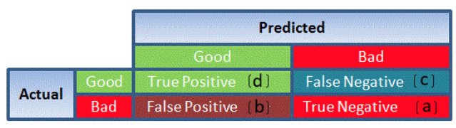
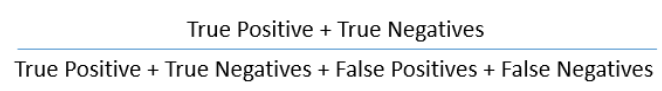
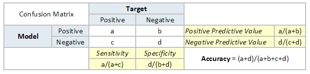
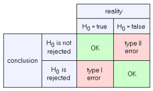
| Accuracy | Accuracy is a metric by which one can examine how good is the machine learning model. Let us look at the confusion matrix to understand it in a better way:
So, the accuracy is the ratio of correctly predicted classes to the total classes predicted. Here, the accuracy will be:
|
| Adam Optimization | The Adam Optimization algorithm is used in training deep learning models. It is an extension to Stochastic Gradient Descent. In this optimization algorithm, running averages of both the gradients and the second moments of the gradients are used. It is used to compute adaptive learning rates for each parameter.
Features:
|
| Apache Spark | Apache Spark is an open-source cluster computing framework. Spark can be deployed in a variety of ways, provides native bindings for the Java, Scala, Python, and R programming languages, and supports SQL, streaming data, and machine learning. Some of the key features of Apache Spark are listed below:
|
| Autoregression | Autoregression is a time series model that uses observations from previous time steps as input to a regression equation to predict the value at the next time step. The autoregressive model specifies that the output variable depends linearly on its own previous values. In this technique input variables are taken as observations at previous time steps, called lag variables.
For example, we can predict the value for the next time step (t+1) given the observations at the last two time steps (t-1 and t-2). As a regression model, this would look as follows: X(t+1) = b0 + b1*X(t-1) + b2*X(t-2) Since the regression model uses data from the same input variable at previous time steps, it is referred to as an autoregression. |
B
Word |
Description |
| Backpropogation | In neural networks, if the estimated output is far away from the actual output (high error), we update the biases and weights based on the error. This weight and bias updating process is known as Back Propagation. Back-propagation (BP) algorithms work by determining the loss (or error) at the output and then propagating it back into the network. The weights are updated to minimize the error resulting from each neuron. The first step in minimizing the error is to determine the gradient (Derivatives) of each node w.r.t. the final output. |
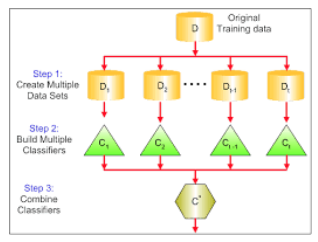
| Bagging | Bagging or bootstrap averaging is a technique where multiple models are created on the subset of data, and the final predictions are determined by combining the predictions of all the models. Some of the algorithms that use bagging technique are :
|
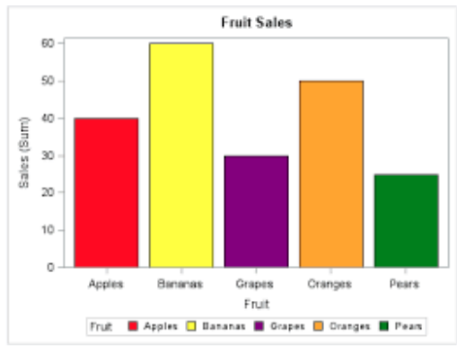
| Bar Chart | Bar charts are a type of graph that are used to display and compare the numbers, frequency or other measures (e.g. mean) for different discrete categories of data. They are used for categorical variables. Simple example of a bar chart:
To gain a better understanding about bar charts, refer here. |
| Bayes Theorem |
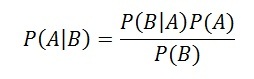
Bayes’ theorem is used to calculate the conditional probability. Conditional probability is the probability of an event ‘B’ occurring given the related event ‘A’ has already occurred. For example, Let’s say a clinic wants to cure cancer of the patients visiting the clinic. A represents an event “Person has cancer” B represents an event “Person is a smoker” The clinic wishes to calculate the proportion of smokers from the ones diagnosed with cancer. To do so use the Bayes’ Theorem (also known as Bayes’ rule) which is as follows: |
| Bayesian Statistics | Bayesian statistics is a mathematical procedure that applies probabilities to statistical problems. It provides people the tools to update their beliefs in the evidence of new data. It differs from classical frequentist approach and is based on the use of Bayesian probabilities to summarize evidence. For more details, read here. |
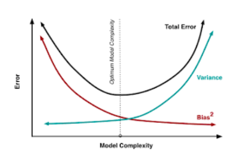
| Bias-Variance Trade-off | The error emerging from any model can be broken down into components mathematically.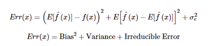
Following are these component :
A high bias error means we have a under-performing model which keeps on missing important trends. A high variance model will over-fit on your training population and perform badly on any observation beyond training. In order to have a perfect fit in the model, the bias and variance should be balanced which is bias variance trade off. |
| Big Data | Big data is a term that describes the large volume of data – both structured and unstructured. But it’s not the amount of data that’s important. It’s how organizations use this large amount of data to generate insights. Companies use various tools, techniques and resources to make sense of this data to derive effective business strategies. |
| Binary Variable | Binary variables are those variables which can have only two unique values. For example, a variable “Smoking Habit” can contain only two values like “Yes” and “No”. |
| Binomial Distribution |
Binomial Distribution is applied only on discrete random variables. It is a method of calculating probabilities for experiments having fixed number of trials. Binomial distribution has following properties:
For a distribution to qualifying as binomial, all of the properties must be satisfied. So, which kind of distributions would be considered binomial? Let’s answer it using few examples:
The formula to calculate probability using Binomial Distribution is: P ( X = r ) = nCr (pˆr)* (1-p) * (n-r) where: |
| Boosting | Boosting is a sequential process, where each subsequent model attempts to correct the errors of the previous model. The succeeding models are dependent on the previous model. Some of the boosting algorithms are:
To learn more about boosting algorithms, refer here. |
| Bootstrapping | Bootstrapping is the process of dividing the dataset into multiple subsets, with replacement. Each subset is of the same size of the dataset. These samples are called bootstrap samples. |
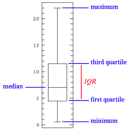
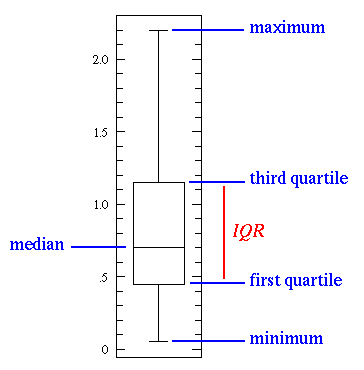
| Box Plot | It displays the full range of variation (from min to max), the likely range of variation (the Interquartile range), and a typical value (the median). Below is a visualization of a box plot:
Some of the inferences that can be made from a box plot:
|
| Business Analytics | Business analytics is mainly used to show the practical methodology followed by an organization for exploring data to gain insights. The methodology focusses on statistical analysis of the data. |
| Business Intelligence | Business intelligence are a set of strategies, applications, data, technologies used by an organization for data collection, analysis and generating insights to derive strategic business opportunities. |
C
Word |
Description |
||||||||||||||||||
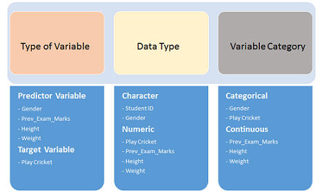
| Categorical Variable | Categorical variables (or nominal variables) are those variables which have discrete qualitative values. For example, names of cities are categorical like Delhi, Mumbai, Kolkata. Read in detail here. | ||||||||||||||||||
| Classification | It is supervised learning method where the output variable is a category, such as “Male” or “Female” or “Yes” and “No”.
For example: Classification Algorithms like Logistic Regression, Decision Tree, K-NN, SVM etc. |
||||||||||||||||||
| Classification Threshold | Classification threshold is the value which is used to classify a new observation as 1 or 0. When we get an output as probabilities and have to classify them into classes, we decide some threshold value and if the probability is above that threshold value we classify it as 1, and 0 otherwise. To find the optimal threshold value, one can plot the AUC-ROC and keep changing the threshold value. The value which will give the maximum AUC will be the optimal threshold value. | ||||||||||||||||||
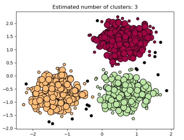
| Clustering |
Clustering is an unsupervised learning method used to discover the inherent groupings in the data. For example: Grouping customers on the basis of their purchasing behaviour which is further used to segment the customers. And then the companies can use the appropriate marketing tactics to generate more profits. Example of clustering algorithms: K-Means, hierarchical clustering, etc. |
||||||||||||||||||
| Computer Vision | Computer Vision is a field of computer science that deals with enabling computers to visualize, process and identify images/videos in the same way that a human vision does. In the recent times, the major driving forces behind Computer Vision has been the emergence of deep learning, rise in computational power and a huge amount of image data. The image data can take many forms, such as video sequences, views from multiple cameras, or multi-dimensional data from a medical scanner. Some of the key applications of Computer Vision are:
|
||||||||||||||||||
| Concordant-Discordant Ratio | Concordant and discordant pairs are used to describe the relationship between pairs of observations. To calculate the concordant and discordant pairs, the data are treated as ordinal. The number of concordant and discordant pairs are used in calculations for Kendall’s tau, which measures the association between two ordinal variables.
Let’s say you had two movie reviewers rank a set of 5 movies:
The ranks given by the reviewer 1 are ordered in ascending order, this way we can compare the rankings given by both the reviewers. Concordant Pair – 2 entities would form a concordant pair if one of them is ranked higher than the other consistently. For example, in the table above B and D form a concordant pair because B has been ranked higher than D by both the reviewers. Discordant Pair – C and D are discordant because they have been ranked in opposite order by the reviewers. Concordant Pair or Discordant Pair ratio = (No. of concordant or discordant pairs) / (Total pairs tested) |
||||||||||||||||||
| Confidence Interval | A confidence interval is used to estimate what percent of a population fits a category based on the results from a sample population. For example, if 70 adults own a cell phone in a random sample of 100 adults, we can be fairly confident that the true percentage amongst the population is somewhere between 61% and 79%. Read more here. | ||||||||||||||||||
| Confusion Matrix |
A confusion matrix is a table that is often used to describe the performance of a classification model. It is a N * N matrix, where N is the number of classes. We form confusion matrix between prediction of model classes Vs actual classes. The 2nd quadrant is called type II error or False Negatives, whereas 3rd quadrant is called type I error or False positives
|
||||||||||||||||||
| Continuous Variable | Continuous variables are those variables which can have infinite number of values but only in a specific range. For example, height is a continuous variable. Read more here. | ||||||||||||||||||
| Convergence | Convergence refers to moving towards union or uniformity. An iterative algorithm is said to converge when as the iterations proceed the output gets closer and closer to a specific value. | ||||||||||||||||||
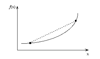
| Convex Function | A real value function is called convex if the line segment between any two points on the graph of the function lies above or on the graph.
Convex functions play an important role in many areas of mathematics. They are especially important in the study of optimization problems where they are distinguished by a number of convenient properties. |
||||||||||||||||||
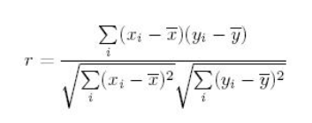
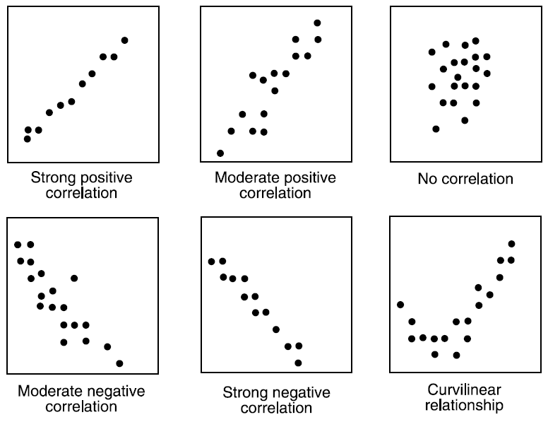
| Correlation | Correlation is the ratio of covariance of two variables to a product of variance (of the variables). It takes a value between +1 and -1. An extreme value on both the side means they are strongly correlated with each other. A value of zero indicates a NIL correlation but not a non-dependence. You’ll understand this clearly in one of the following answers.
The most widely used correlation coefficient is Pearson Coefficient. Here is the mathematical formula to derive Pearson Coefficient.
|
||||||||||||||||||
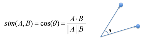
| Cosine Similarity | Cosine Similarity is the cosine of the angle between 2 non-zero vectors. Two parallel vectors have a cosine similarity of 1 and two vectors at 90° have a cosine similarity of 0. Suppose we have two vectors A and B, cosine similarity of these vectors can be calculated by dividing the dot product of A and B with the product of the magnitude of the two vectors.
|
||||||||||||||||||
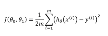
| Cost Function | Cost function is used to define and measure the error of the model. The cost function is given by:
Here,
Let us understand it with an example: So let’s say, you increase the size of a particular shop, where you predicted that the sales would be higher. But despite increasing the size, the sales in that shop did not increase that much. So the cost applied in increasing the size of the shop, gave you negative results. So, we need to minimize these costs. Therefore we make use of cost function to minimize the loss. |
||||||||||||||||||
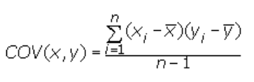
| Covariance | Covariance is a measure of the joint variability of two random variables. It’s similar to variance, but where variance tells you how a single variable varies, co variance tells you how two variables vary together. The formula for covariance is:
Where, x = the independent variable y = the dependent variable n = number of data points in the sample x bar = the mean of the independent variable x y bar = the mean of the dependent variable y A positive covariance means the variables are positively related, while a negative covariance means the variables are inversely related. |
||||||||||||||||||
| Cross Entropy | In information theory, the cross entropy between two probability distributions and over the same underlying set of events measures the average number of bits needed to identify an event drawn from the set, if a coding scheme is used that is optimized for an “unnatural” probability distribution , rather than the “true”. Cross entropy can be used to define the loss function in machine learning and optimization. | ||||||||||||||||||
| Cross Validation | Cross Validation is a technique which involves reserving a particular sample of a dataset which is not used to train the model. Later, the model is tested on this sample to evaluate the performance. There are various methods of performing cross validation such as:
|

D
Word |
Description |
||||||||
| Data Mining | Data mining is a study of extracting useful information from structured/unstructured data taken from various sources. This is done usually for
Data Mining is done for purposes like Market Analysis, determining customer purchase pattern, financial planning, fraud detection, etc |
||||||||
| Data Science | Data science is a combination of data analysis, algorithmic development and technology in order to solve analytical problems. The main goal is a use of data to generate business value. | ||||||||
| Data Transformation |
Data transformation is the process to convert data from one form to the other. This is usually done at a preprocessing step.
For instance, replacing a variable x by the square root of x
|
||||||||
| Database | Database (abbreviated as DB) is an structured collection of data. The collected information is organised in a way such that it is easily accessible by the computer. Databases are built and managed by using database programming languages. The most common database language is SQL. | ||||||||
| Dataframe | DataFrame is a 2-dimensional labeled data structure with columns of potentially different types. You can think of it like a spreadsheet or SQL table, or a dict of Series objects. DataFrame accepts many different kinds of input:
|
||||||||
| Dataset | A dataset (or data set) is a collection of data. A dataset is organized into some type of data structure. In a database, for example, a dataset might contain a collection of business data (names, salaries, contact information, sales figures, and so forth). Several characteristics define a dataset’s structure and properties. These include the number and types of the attributes or variables, and various statistical measures applicable to them, such as standard deviation and kurtosis. | ||||||||
| Dashboard | Dashboard is an information management tool which is used to visually track, analyze and display key performance indicators, metrics and key data points. Dashboards can be customised to fulfil the requirements of a project. It can be used to connect files, attachments, services and APIs which is displayed in the form of tables, line charts, bar charts and gauges. Popular tools for building dashboards include Excel and Tableau. | ||||||||
| DBScan | DBSCAN is the acronym for Density-Based Spatial Clustering of Applications with Noise. It is a clustering algorithm that isolates different density regions by forming clusters. For a given set of points, it groups the points which are closely packed.
The algorithm has two important features:
The steps involved in this algorithm are:
The below image is an example of DBScan on a set of normalized data points:
|
||||||||
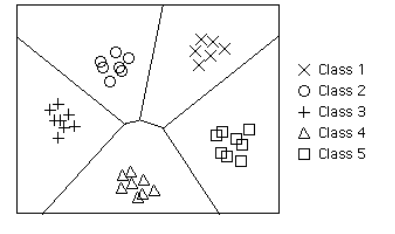
| Decision Boundary | In a statistical-classification problem with two or more classes, a decision boundary or decision surface is a hypersurface that partitions the underlying vector space into two or more sets, one for each class. How well the classifier works depends upon how closely the input patterns to be classified resemble the decision boundary. In the example sketched below, the correspondence is very close, and one can anticipate excellent performance.
Here the lines separating each class are decision boundaries. |
||||||||
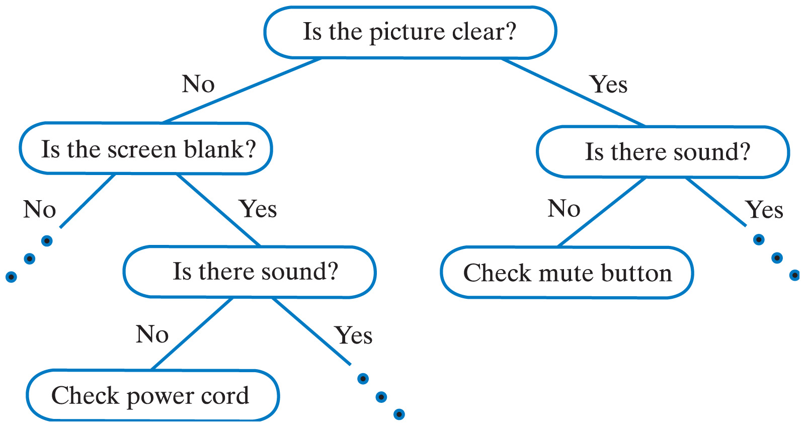
| Decision Tree |
Decision tree is a type of supervised learning algorithm (having a pre-defined target variable) that is mostly used in classification problems. It works for both categorical and continuous input & output variables. In this technique, we split the population (or sample) into two or more homogeneous sets (or sub-populations) based on most significant splitter / differentiator in input variables.
Read more here. |
||||||||
| Deep Learning | Deep Learning is associated with a machine learning algorithm (Artificial Neural Network, ANN) which uses the concept of human brain to facilitate the modeling of arbitrary functions. ANN requires a vast amount of data and this algorithm is highly flexible when it comes to model multiple outputs simultaneously. To understand ANN in detail, read here. | ||||||||
| Descriptive Statistics | Descriptive statistics is comprised of those values which explains the spread and central tendency of data. For example, mean is a way to represent central tendency of the data, whereas IQR is a way to represent spread of the data. | ||||||||
| Dependent Variable | A dependent variable is what you measure and which is affected by independent / input variable(s). It is called dependent because it “depends” on the independent variable. For example, let’s say we want to predict the smoking habits of people. Then the person smokes “yes” or “no” is the dependent variable. | ||||||||
| Decile | Decile divides a series into 10 equal parts. For any series, there are 10 decile denoted by D1, D2, D3 … D10. These are known as First Decile , Second Decile and so on.
For example, the diagram below shows the health score of a patient from range 0 to 60. Nine deciles split the patients into 10 groups
|
||||||||
| Degree of Freedom | It is the number of variables that have the choice of having more than one arbitrary value.
For example, in a sample of size 10 with mean 10, 9 values can be arbitrary but the 10th value is forced by the sample mean. So, we can choose any number for 9 values but the 10th value must be such that the mean is 10. So, the degree of freedom in this case will be 9. |
||||||||
| Dimensionality Reduction | Dimensionality Reduction is the process of reducing the number of random variables under consideration by obtaining a set of principal variables. Dimension Reduction refers to the process of converting a set of data having vast dimensions into data with lesser dimensions ensuring that it conveys similar information concisely. Some of the benefits of dimensionality reduction:
|
||||||||
| Dplyr | Dplyr is a popular data manipulation package in R. It makes data manipulation, cleaning, summarizing very user friendly. Dplyr can work not only with the local datasets, but also with remote database tables, using exactly the same R code.
It can be easily installed using the following code from the R console: install.packages("dplyr") |
||||||||
| Dummy Variable | Dummy Variable is another name for Boolean variable. An example of dummy variable is that it takes value 0 or 1. 0 means value is true (i.e. age < 25) and 1 means value is false (i.e. age >= 25) |
E
Word |
Description |
| Early Stopping | Early stopping is a technique for avoiding overfitting when training a machine learning model with iterative method. We set the early stopping in such a way that when the performance has stopped improving on the held-out validation set, the model training stops.
For example, in XGBoost, as you train more and more trees, you will overfit your training dataset. Early stopping enables you to specify a validation dataset and the number of iterations after which the algorithm should stop if the score on your validation dataset didn’t increase. |
| EDA | EDA or exploratory data analysis is a phase used for data science pipeline in which the focus is to understand insights of the data through visualization or by statistical analysis.
The steps involved in EDA are:
Refer here for a comprehensive guide to doing EDA. |
| ETL | ETL is the acronym for Extract, Transform and Load. An ETL system has the following properties:
This data can be used by application developers to build applications and end users for making decisions. |
| Evaluation Metrics` |
The purpose of evaluation metric is to measure the quality of the statistical / machine learning model. For example, below are a few evaluation metrics
|
F
Word |
Description |
||||||||||||||||||||
| Factor Analysis | Factor analysis is a technique that is used to reduce a large number of variables into fewer numbers of factors. Factor analysis aims to find independent latent variables. Factor analysis also assumes several assumptions:
There are different types of methods used to extract the factor from the data set:
|
||||||||||||||||||||
| False Negative | Points which are actually true but are incorrectly predicted as false. For example, if the problem is to predict the loan status. (Y-loan approved, N-loan not approved). False negative in this case will be the samples for which loan was approved but the model predicted the status as not approved. | ||||||||||||||||||||
| False Positive | Points which are actually false but are incorrectly predicted as true. For example, if the problem is to predict the loan status. (Y-loan approved, N-loan not approved). False positive in this case will be the samples for which loan was not approved but the model predicted the status as approved. | ||||||||||||||||||||
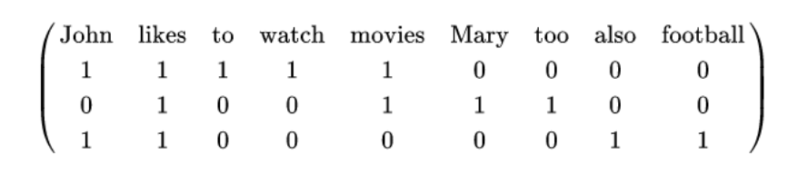
| Feature Hashing |
It is a method to transform features to vector. Without looking up the indices in an associative array, it applies a hash function to the features and uses their hash values as indices directly. Simple example of feature hashing:
Suppose we have three documents:
Now we can convert this to vector using hashing.
The array form for the same will be:
|
||||||||||||||||||||
| Feature Reduction | Feature reduction is the process of reducing the number of features to work on a computation intensive task without losing a lot of information.
PCA is one of the most popular feature reduction techniques, where we combine correlated variables to reduce the features.
|
||||||||||||||||||||
| Feature Selection |
Feature Selection is a process of choosing those features which are required to explain the predictive power of a statistical model and dropping out irrelevant features.
This can be done by either filtering out less useful features or by combining features to make a new one.
Refer here. |
||||||||||||||||||||
| Few-shot Learning |
Few-shot learning refers to the training of machine learning algorithms using a very small set of training data instead of a very large set. This is most suitable in the field of computer vision, where it is desirable to have an object categorization model work well without thousands of training examples. | ||||||||||||||||||||
| Flume | Flume is a service designed for streaming logs into the Hadoop environment. It can collect and aggregate huge amounts of log data from a variety of sources. In order to collect high volume of data, multiple flume agents can be configured.
Here are the major features of Apache Flume:
|
||||||||||||||||||||
| Frequentist Statistics |
Frequentist Statistics tests whether an event (hypothesis) occurs or not. It calculates the probability of an event in the long run of the experiment (i.e the experiment is repeated under the same conditions to obtain the outcome). Here, the sampling distributions of fixed size are taken. Then, the experiment is theoretically repeated infinite number of times but practically done with a stopping intention. For example, I perform an experiment with a stopping intention in mind that I will stop the experiment when it is repeated 1000 times or I see minimum 300 heads in a coin toss. Read more here. |
||||||||||||||||||||
| F-Score | F-score evaluation metric combines both precision and recall as a measure of effectiveness of classification. It is calculated in terms of ratio of weighted importance on either recall or precision as determined by β coefficient.
F measure = 2 x (Recall × Precision) / ( β² × Recall + Precision ) |

G
Word |
Description |
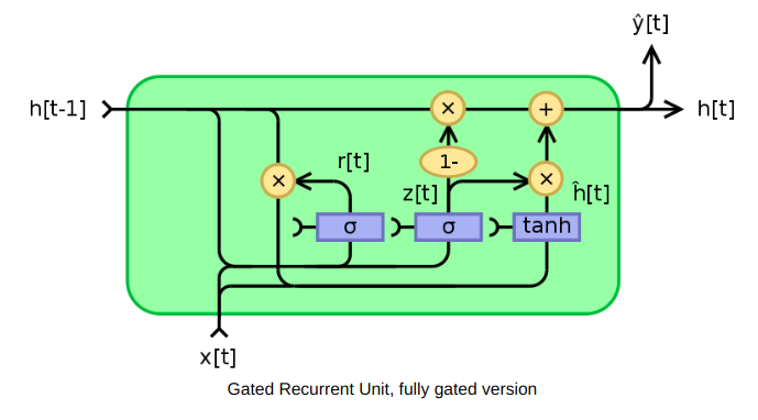
| Gated Recurrent Unit (GRU) | The GRU is a variant of the LSTM (Long Short Term Memory) and was introduced by K. Cho. It retains the LSTM’s resistance to the vanishing gradient problem, but because of its simpler internal structure it is faster to train.
Instead of the input, forget, and output gates in the LSTM cell, the GRU cell has only two gates, an update gate z, and a reset gate r. The update gate defines how much previous memory to keep, and the reset gate defines how to combine the new input with the previous memory.
|
| Ggplot2 | GGplot2 is a data visualization package for the R programming language. It is a highly versatile and user-friendly tool for creating attractive plots. To know more about Ggplot2, visit here.
It can be easily installed using the following code from the R console: install.packages("ggplot2") |
| Go | Go is an open source programming language that makes it easy to build simple, reliable, and efficient software. Go is a statically typed language in the tradition of C.
The main features of Go are:
The compiler and other tools originally developed by Google are all free and open source. To read further on the Go language, refer here. |
| Goodness of Fit | The goodness of fit of a model describes how well it fits a set of observations. Measures of goodness of fit typically summarize the discrepancy between observed values and the values expected under the model.
With regard to a machine learning algorithm, a good fit is when the error for the model on the training data as well as the test data is minimum. Over time, as the algorithm learns, the error for the model on the training data goes down and so does the error on the test dataset. If we train for too long, the performance on the training dataset may continue to decrease because the model is overfitting and learning the irrelevant detail and noise in the training dataset. At the same time the error for the test set starts to rise again as the model’s ability to generalize decreases. So the point just before the error on the test dataset starts to increase where the model has good skill on both the training dataset and the unseen test dataset is known as the good fit of the model. |
| Gradient Descent | Gradient descent is a first-order iterative optimization algorithm for finding the minimum of a function. In machine learning algorithms, we use gradient descent to minimize the cost function. It find out the best set of parameters for our algorithm. Gradient Descent can be classified as follows:
In full batch gradient descent algorithms, we use whole data at once to compute the gradient, whereas in stochastic we take a sample while computing the gradient.
|
H
Word |
Description |
| Hadoop | Hadoop is an open source distributed processing framework used when we have to deal with enormous data. It allows us to use parallel processing capability to handle big data. Here are some significant benefits of Hadoop:
|
| Hidden Markov Model | Hidden Markov Process is a Markov process in which the states are invisible or hidden, and the model developed to estimate these hidden states is known as the Hidden Markov Model (HMM). However, the output (data) dependent on the hidden states is visible. This output data generated by HMM gives some cue about the sequence of states.
HMM are widely used for pattern recognition in speech recognition, part-of-speech tagging, handwriting recognition, and reinforcement learning. |
| Hierarchical Clustering |
Hierarchical clustering, as the name suggests is an algorithm that builds hierarchy of clusters. This algorithm starts with all the data points assigned to a cluster of their own. Then two nearest clusters are merged into the same cluster. In the end, this algorithm terminates when there is only a single cluster left. The results of hierarchical clustering can be shown using dendrogram. The dendrogram can be interpreted as:
Read more here. |
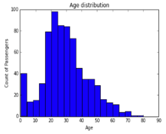
| Histogram | Histogram is one of the methods for visualizing data distribution of continuous variables. For example, the figure below shows a histogram with age along the x-axis and frequency of the variable (count of passengers) along the y-axis.
Histograms are widely used to determine the skewness of the data. Looking at the tail of the plot, you can find whether the data distribution is left skewed, normal or right skewed.
|
| Hive | Hive is a data warehouse software project to process structured data in Hadoop. It is built on top of Apache Hadoop for providing data summarization, query and analysis. Hive gives an SQL-like interface to query data stored in various databases and file systems that integrate with Hadoop. Some of the key features of Hive are :
For detailed information, refer here. |
| Holdout Sample | While working on the dataset, a small part of the dataset is not used for training the model instead, it is used to check the performance of the model. This part of the dataset is called the holdout sample.
For instance, if I divide my data in two parts – 7:3 and use the 70% to train the model, and other 30% to check the performance of my model, the 30% data is called the holdout sample. |
| Holt-Winters Forecasting | Holt-Winters is one of the most popular forecasting techniques for time series. The model predicts the future values computing the combined effects of both trend and seasonality. The idea behind Holt’s Winter forecasting is to apply exponential smoothing to the seasonal components in addition to level and trend.
Visit here for more details. |
| Hyperparameter | A hyperparameter is a parameter whose value is set before training a machine learning or deep learning model. Different models require different hyperparameters and some require none. Hyperparameters should not be confused with the parameters of the model because the parameters are estimated or learned from the data.
Some keys points about the hyperparameters are:
Number of trees in a Random Forest, eta in XGBoost, and k in k-nearest neighbours are some examples of hyperparameters. |
| Hyperplane | It is a subspace with one fewer dimensions than its surrounding area. If a space is 3-dimensional then its hyperplane is just a normal 2D plane. In 5 dimensional space, it’s a 4D plane, so on and so forth.
Most of the time it’s basically a normal plane, but in some special cases, like in Support Vector Machines, where classifications are performed with an n-dimensional hyperplane, the n can be quite large. |
| Hypothesis | Simply put, a hypothesis is a possible view or assertion of an analyst about the problem he or she is working upon. It may be true or may not be true. Read more here. |
I
Word |
Description |
||||||||||||||||
| Imputation | Imputation is a technique used for handling missing values in the data. This is done either by statistical metrics like mean/mode imputation or by machine learning techniques like kNN imputation
For example, If the data is as below
The second row contains a missing value, so to impute it we use mean of all ages, i.e.
|
||||||||||||||||
| Inferential Statistics | In inferential statistics, we try to hypothesize about the population by only looking at a sample of it. For example, before releasing a drug in the market, internal tests are done to check if the drug is viable for release. But here we cannot check with the whole population for viability of the drug, so we do it on a sample which best represents the population. | ||||||||||||||||
| IQR | IQR (or interquartile range) is a measure of variability based on dividing the rank-ordered data set into four equal parts. It can be derived by Quartile3 – Quartile1.
|
||||||||||||||||
| Iteration | Iteration refers to the number of times an algorithm’s parameters are updated while training a model on a dataset. For example, each iteration of training a neural network takes certain number of training data and updates the weights by using gradient descent or some other weight update rule. |
J
Word |
Description |
| Julia | Julia is a high-level, high-performance dynamic programming language for numerical computing. Some important features of Julia are:
|
K
Word |
Description |
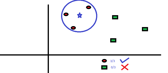
| K-Means |
It is a type of unsupervised algorithm which solves the clustering problem. It is a procedure which follows a simple and easy way to classify a given data set through a certain number of clusters (assume k clusters). Data points inside a cluster are homogeneous and heterogeneous to peer groups.
|
| Keras | Keras is a simple, high-level neural network library, written in Python. It is capable of running on top of Tensorflow and Theano. This is done to make design and experiments with Neural Networks easier.
Following are some important features of Keras:
|
| kNN |
K nearest neighbors is a simple algorithm that stores all available cases and classifies new cases by a majority vote of its k neighbors. The case being assigned to the class is most common amongst its K nearest neighbors measured by a distance function. These distance functions can be Euclidean, Manhattan, Minkowski and Hamming distance. First three functions are used for continuous function and fourth one (Hamming) for categorical variables. If K = 1, then the case is simply assigned to the class of its nearest neighbor. At times, choosing the value for K can be a challenge while performing KNN modeling.
|
| Kurtosis |
Kurtosis is defined as the thickness (or heaviness) of the tails of a given distribution. Depending on the value of kurtosis, it can be classified into the below 3 categories:
|

L
Word |
Description |
| Labeled Data | A labeled dataset has a meaningful “label”, “class” or “tag” associated with each of its records or rows. For example, labels for a dataset of a set of images might be whether an image contains a cat or a dog.
Labeled data are usually more expensive to obtain than the raw unlabeled data because preparation of the labelled data involves manual labelling every piece of unlabeled data. Labeled data is required for supervised learning algorithms. |
| Lasso Regression |
Lasso regression performs L1 regularization, i.e. it adds a factor of sum of absolute value of coefficients in the optimization objective. Thus, lasso regression optimizes the following: Objective = RSS + α * (sum of absolute value of coefficients)Here, α (alpha) works similar to that of ridge and provides a trade-off between balancing RSS and magnitude of coefficients. Like that of ridge, α can take various values. Let’s iterate it briefly here:
|
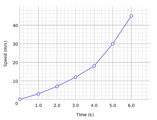
| Line Chart | Line charts are used to display information as series of points connected by straight line segment. These charts are used to communicate information visually, such as to show an increase or decrease in the trend in data over intervals of time.
In the plot below, for each time instance, the speed trend is shown and the points are connected to display the trend over time.
This plot is for a single case. Line charts can also be used to compare changes over the same period of time for multiple cases, like plotting the speed of a cycle, car, train over time in the same plot. |
| Linear Regression |
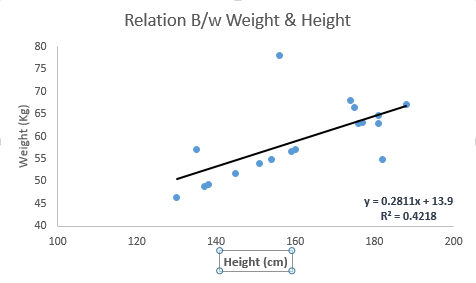
The best way to understand linear regression is to relive this experience of childhood. Let us say, you ask a child in fifth grade to arrange people in his class by increasing order of weight, without asking them their weight! What do you think the child will do? He / she would likely look (visually analyze) at the height and build of people and arrange them using a combination of these visible parameters. This is linear regression in real life. The child has actually figured out that height and build would be correlated to the weight by a relationship, which looks like the equation below. Y=aX+b where:
These coefficients a and b are derived based on minimizing the sum of squared difference of distance between data points and regression line. Look at the below example. Here we have identified the best fit line having linear equation y=0.2811x+13.9. Now using this equation, we can find the weight, knowing the height of a person.
|
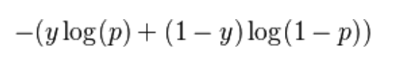
| Log Loss | Log Loss or Logistic loss is one of the evaluation metrics used to find how good the model is. Lower the log loss, better is the model. Log loss is the logarithm of the product of all probabilities.
Mathematically, log loss for two classes is defined as:
where, y is the class label and p is the predicted probability. |
| Logistic Regression | In simple words, it predicts the probability of occurrence of an event by fitting data to a logistic function. Hence, it is also known as logistic regression. Since, it predicts the probability, the output values lies between 0 and 1 (as expected). |
| Long Short Term Memory (LSTM) | Long short-term memory (LSTM) units (or blocks) are a building unit for layers of a recurrent neural network (RNN). A common LSTM unit is composed of a cell, an input gate, an output gate and a forget gate. The cell is responsible for “remembering” values over arbitrary time intervals, hence the word “memory” in LSTM. Each of the three gates can be thought of as a “conventional” artificial neuron, as in a multi-layer neural network, that is, they compute an activation (using an activation function) of a weighted sum. Applications of LSTM include:
To learn further on LSTM, refer here. |
M
Word |
Description |
||||||||||||||||
| Machine Learning | Machine Learning refers to the techniques involved in dealing with vast data in the most intelligent fashion (by developing algorithms) to derive actionable insights. In these techniques, we expect the algorithms to learn by itself wiithout being explicitly programmed. | ||||||||||||||||
| Mahout | Mahout is an open source project from Apache that is used for creating scalable machine learning algorithms. It implements popular machine learning techniques such as recommendation, classification, clustering.
Features of Mahout:
|
||||||||||||||||
| MapReduce | Hadoop MapReduce is a software framework for easily writing applications which process vast amounts of data (multi-terabyte data-sets) in-parallel on large clusters (thousands of nodes) of commodity hardware in a reliable, fault-tolerant manner.
A MapReduce framework is usually composed of three operations:
To learn more about MapReduce, visit here. |
||||||||||||||||
| Market Basket Analysis | Market Basket Analysis (also called as MBA) is a widely used technique among the Marketers to identify the best possible combinatory of the products or services which are frequently bought by the customers. This is also called product association analysis.Association analysis mostly done based on an algorithm named “Apriori Algorithm”. The Outcome of this analysis is called association rules. Marketers use these rules to strategize their recommendations.
When two or more products are purchased, Market Basket Analysis is done to check whether the purchase of one product increases the likelihood of the purchase of other products. This knowledge is a tool for the marketers to bundle the products or strategize a product cross sell to a customer. |
||||||||||||||||
| Market Mix Modeling | Market Mix Modeling is an analytical approach that uses historical information like point of sales to quantify the impact of some of the components on sales.
Suppose the total sale is 100$, this total can be broken into sub components i.e. 60$ base sale, 20$ pricing, 18$ may be distribution and 2$ might be due to promotional activity. These numbers can be achieved using various logical methods. Every method can give a different break up. Hence, it becomes very important to standardize the process of breaking up the total sales into these components. This formal technique is formally known as MMM or Market Mix Modeling. |
||||||||||||||||
| Maximum Likelihood Estimation | It is a method for finding the values of parameters which make the likelihood maximum. The resulting values are called maximum likelihood estimates (MLE). | ||||||||||||||||
| Mean | For a dataset, mean is said to be the average value of all the numbers. It can sometimes be used as a representation of the whole data.
For instance, if you have the marks of students from a class, and you asked about how good is the class performing. It would be irrelevant to say the marks of every single student, instead, you can find the mean of the class, which will be a representative for class performance. For example, if the numbers are 1,2,3,4,5,6,7,8,8 then the mean would be 44/9 = 4.89. |
||||||||||||||||
| Median | Median of a set of numbers is usually the middle value. When the total numbers in the set are even, the median will be the average of the two middle values. Median is used to measure the central tendency.
To calculate the median for a set of numbers, follow the below steps:
|
||||||||||||||||
| MIS | A management information system (MIS) is a computer system consisting of hardware and software that serves as the backbone of an organization’s operations. An MIS gathers data from multiple online systems, analyzes the information, and reports data to aid in management decision-making.
Objectives of MIS:
|
||||||||||||||||
| ML-as-a-Service (MLaaS) | Machine learning as a service (MLaaS) is an array of services that provide machine learning tools as part of cloud computing services. This can include tools for data visualization, facial recognition, natural language processing, image recognition, predictive analytics, and deep learning. Some of the top ML-as-a-service providers are:
|
||||||||||||||||
| Mode | Mode is the most frequent value occuring in the population. It is a metric to measure the central tendency, i.e. a way of expressing, in a (usually) single number, important information about a random variable or a population.
Mode can be calculated using following steps:
Let us understand it with an example: Suppose we have a dataset having 10 data points, listed below: 4,5,2,8,4,7,6,4,6,3 So now we will calculate the number of times each value has appeared.
So we see that the value 4 is repeating the most, i.e., 3 times. So, the mode of this dataset will be 4. |
||||||||||||||||
| Model Selection | Model selection is the task of selecting a statistical model from a set of known models. Various methods that can be used for choosing the model are:
Some of the criteria for selecting the model can be:
|
||||||||||||||||
| Monte Carlo Simluation | The idea behind Monte Carlo Simulation is to use random samples of parameters or inputs to explore the behavior of a complex process. Monte Carlo simulations sample from a probability distribution for each variable to produce hundreds or thousands of possible outcomes. The results are analyzed to get probabilities of different outcomes occurring. | ||||||||||||||||
| Multi-Class Classification | Problems which have more than one class in the target variable are called multi-class Classification problems.
For example, if the target is to predict the quality of a product, which can be Excellent, good, average, fair, bad. In this case, the variable has 5 classes, hence it is a 5-class classification problem. |
||||||||||||||||
| Multivariate Analysis | Multivariate analysis is a process of comparing and analyzing the dependency of multiple variables over each other.
For example, we can perform bivariate analysis of combination of two continuous features and find a relationship between them.
|
||||||||||||||||
| Multivariate Regression | Multivariate, as the word suggests, refers to ‘multiple dependent variables’. A regression model designed to deal with multiple dependent variables is called a multivariate regression model.
Consider the example – for a given set of details about a student’s interests, previous subject-wise score etc, you want to predict the GPA for all the semesters (GPA1, GPA2, …. ). This problem statement can be addressed using multivariate regression since we have more than one dependent variable. |
N
Word |
Description |
| Naive Bayes | It is a classification technique based on Bayes’ theorem with an assumption of independence between predictors. In simple terms, a Naive Bayes classifier assumes that the presence of a particular feature in a class is unrelated to the presence of any other feature. For example, a fruit may be considered to be an apple if it is red, round and about 3 inches in diameter. Even if these features depend on each other or upon the existence of the other features, a naive Bayes classifier would consider all of these properties to independently contribute to the probability that this fruit is an apple. |
| NaN | NaN stands for ‘not a number’. It is a numeric data type value representing an undefined or unrepresentable value. If the dataset has NaN values somewhere, it means that the data at that location is either missing or represented incorrectly. |
| Natural Language Processing | In simple words, Natural Language Processing is a field which aims to make computer systems understand human speech. NLP is comprised of techniques to process, structure, categorize raw text and extract information.
ChatBot is a classic example of NLP, where sentences are first processed, cleaned and converted to machine understandable format. |
| NoSQL | NoSQL means Not only SQL. A NoSQL database provides a mechanism for storage and retrieval of data that is modeled in means other than the tabular relations used in relational databases. It can accommodate a wide variety of data models, including key-value, document, columnar and graph formats.
Types of NoSQL:
To learn more about NoSQL and its types, refer here. |
| Nominal Variable | Nominal variables are categorical variables having two or more categories without any kind of order to them.
For example, a column called “name of cities” with values such as Delhi, Mumbai, Chennai, etc. We can see that there is no order between the variables – viz Delhi is in no particular way higher or lower than Mumbai (unless explicitly mentioned). |
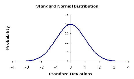
| Normal Distribution |
The normal distribution is the most important and most widely used distribution in statistics. It is sometimes called the bell curve, because it has a peculiar shape of a bell. Mostly, a binomial distribution is similar to normal distribution. The difference between the two is normal distribution is continuous.
|
| Normalization | Normalization is the process of rescaling your data so that they have the same scale. Normalization is used when the attributes in our data have varying scales.
For example, if you have a variable ranging from 0 to 1 and other from 0 to 1000, you can normalize the variable, such that both are in the range 0 to 1. |
| Numpy | NumPy is the fundamental package for scientific computing with Python. It contains among other things:
Besides its obvious scientific uses, NumPy can also be used as an efficient multi-dimensional container of generic data. Arbitrary data-types can be defined. This allows NumPy to seamlessly and speedily integrate with a wide variety of databases. |
O
Word |
Description |
||||||||||||||||||||||||
| One Hot Encoding |
One Hot encoding is done usually in the preprocessing step. It is a technique which converts categorical variables to numerical in an interpretable format. In this we create a Boolean column for each category of the variable.
For example, if the data is
This is converted as
|
||||||||||||||||||||||||
| One Shot Learning | It is a machine learning approach where the model is trained on a single example. One-shot Learning is generally used for object classification. This is performed to design effective classifiers from a single training example. | ||||||||||||||||||||||||
| Oozie | Apache Oozie is the tool in which all sort of programs can be pipelined in a desired order to work in Hadoop’s distributed environment. Oozie also provides a mechanism to run the job at a given schedule.
It consists of two parts:
Features of Oozie:
|
||||||||||||||||||||||||
| Ordinal Variable | Ordinal variables are those variables which have discrete values but has some order involved. Refer here. | ||||||||||||||||||||||||
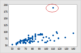
| Outlier | Outlier is an observation that appears far away and diverges from an overall pattern in a sample.
|
||||||||||||||||||||||||
| Overfitting | A model is said to overfit when it performs well on the train dataset but fails on the test set. This happens when the model is too sensitive and captures random patterns which are present only in the training dataset. There are two methods to overcome overfitting:
|
P
Word |
Description |
| Pandas | Pandas is an open source, high-performance, easy-to-use data structure and data analysis library for the Python programming language. Some of the highlights of Pandas are:
For more information on Pandas, you can refer here. |
| Parameters | Parameters are a set of measurable factors that define a system. For machine learning models, model parameters are internal variables whose values can be determined from the data.
For instance, the weights in linear and logistic regression fall under the category of parameters. |
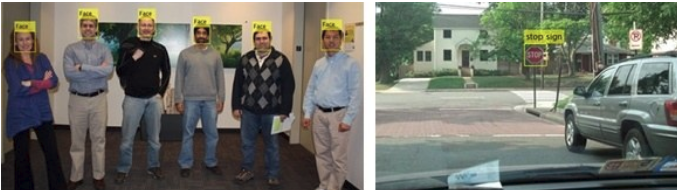
| Pattern Recognition | Pattern recognition is a branch of machine learning that focuses on the recognition of patterns and regularities in data. Classification is an example of pattern recognition wherein each input value is assigned one of a given set of classes.
In computer vision, supervised pattern recognition techniques are used for optical character recognition (OCR), face detection, face recognition, object detection, and object classification.
|
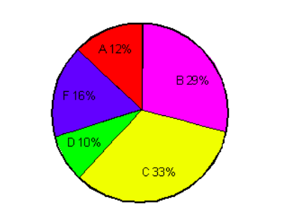
| Pie Chart | A pie chart is a circular statistical graphic which is divided into slices to illustrate numerical proportion. The arc length of each slice, is proportional to the quantity it represents. Let us understand it with an example:
This represents a pie graph showing the results of an exam. Each grade is denoted by a “slice”. The total of the percentages is equal to 100. The total of the arc measures is equal to 360 degrees. So 12% students got A grade, 29% got B, and so on. |
| Pig | Pig is a high level scripting language that is used with Apache Hadoop. Pig enables data workers to write complex data transformations without knowing Java. Pig is complete, so one can do all required data manipulations in Apache Hadoop with Pig. Through the User Defined Functions(UDF) facility in Pig, Pig can invoke code in many languages like JRuby, Jython and Java.
Key features of Pig:
To read further on Pig, refer here. |
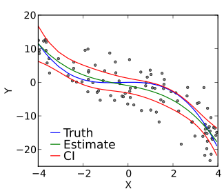
| Polynomial Regression |
In this technique, a curve fits into the data points. In a polynomial regression equation, the power of the independent variable is greater than 1. Although higher degree polynomials give lower error, they might also result in over-fitting.
|
| Pre-trained Model |
A pre-trained model is a model created by someone else to solve a similar problem. Instead of building a model from scratch to solve a similar problem, you use the model trained on other problem as a starting point.
For example, if you want to build a self learning car. You can spend years to build a decent image recognition algorithm from scratch or you can take inception model (a pre-trained model) from Google which was built on ImageNet data to identify images in those pictures. For more information regarding Pre-trained model and their usages, you can refer here.
|
| Precision and Recall |
Precision can be measured as of the total actual positive cases, how many positives were predicted correctly.
It can be represented as: Precision = TP / (TP + FP) Whereas recall is described as the measured of how many of the positive predictions were correct. It can be represented as: Recall = TP / (TP + FN)
|
| Predictor Variable | Predictor variable is used to make a prediction for dependent variables. |
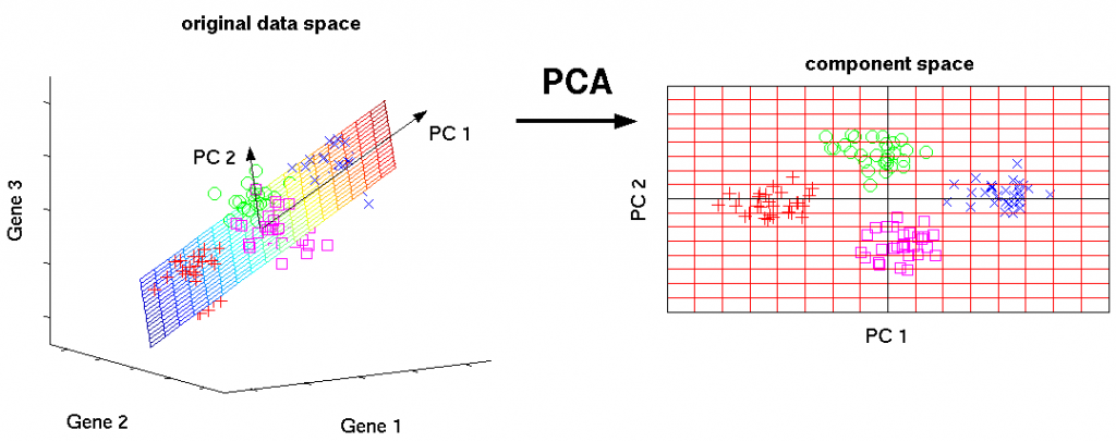
| Principal Component Analysis (PCA) | Principal component analysis (PCA) is an approach to factor analysis that considers the total variance in the data, and transforms the original variables into a smaller set of linear combinations. PCA is sensitive to outliers; they should be removed.
It is a statistical procedure that uses an orthogonal transformation to convert a set of observations of possibly correlated variables into a set of values of linearly uncorrelated variables called principal components. PCA is mostly used as a tool in exploratory data analysis and for making predictive models. It’s often used to visualize genetic distance and relatedness between populations. |
| P-Value | P-value is the value of probability of getting a result equal to or greater than the observed value, when the null hypothesis is true. |
| Python | Python is an open source programming language, widely used for various applications, such as general purpose programming, data science and machine learning. Usually preferred by beginners in these fields because of the following major advantages:
To learn python from scratch, you can follow this article. |
| PyTorch | PyTorch is an open source machine learning library for python, based on Torch. It is built to provide flexibility as a deep learning development platform. Here are a few reasons for which PyTorch is extensively used :
|

Q
Word |
Description |
| Quartile |
Quartile divides a series into 4 equal parts. For any series, there are 4 quartiles denoted by Q1, Q2, Q3 and Q4. These are known as First Quartile , Second Quartile and so on. For example, the diagram below shows the health score of a patient from range 0 to 60. Quartiles divide the population into 4 groups.
|
R
Word |
Description |
| R | R is an open-source programming language and a software environment for statistical computing, machine learning, and data visualization.
Features of R:
|
| Range | Range is the difference between the highest and the lowest value of the population. It is used to measure the spread of the data.Let us understand it with an example:
Suppose we have a dataset having 10 data points, listed below: 4,5,2,8,4,7,6,4,6,3 So, first of all we will arrange these data points in ascending order: 2,3,4,4,4,5,6,6,7,8 Now the range of this set is the difference between the highest(8) and the lowest(2) value. Range = 8-2 = 6 |
| Recommendation Engine | Generally people tend to buy products recommended to them by their friends or the people they trust. Nowadays in the digital age, any online shop you visit utilizes some sort of recommendation engine. Recommendation engines basically are data filtering tools that make use of algorithms and data to recommend the most relevant items to a particular user. If we can recommend items to a customer based on their needs and interests, it will create a positive effect on the user experience and they will visit more frequently. There are few types of recommendation engines:
|
| Regression |
It is supervised learning method where the output variable is a real value, such as “amount” or “weight”. Example of Regression: Linear Regression, Ridge Regression, Lasso Regression |
| Regression Spline | Regression Splines is a non-linear approach that uses a combination of linear/polynomial functions to fit the data. In this technique, instead of building one model for the entire dataset, it is divided into multiple bins and a separate model is built on each bin.
Read more about this topic here. |
| Regularization | Regularization is a technique used to solve the overfitting problem in statistical models. In machine learning, regularization penalizes the coefficients such that the model generalize better. We have different types of regression techniques which uses regularization such as Ridge regression and lasso regression.
|
| Reinforcement Learning |
It is an example of machine learning where the machine is trained to take specific decisions based on the business requirement with the sole motto to maximize efficiency (performance). The idea involved in reinforcement learning is: The machine/ software agent trains itself on a continual basis based on the environment it is exposed to, and applies it’s enriched knowledge to solve business problems. This continual learning process ensures less involvement of human expertise which in turn saves a lot of time! Important Note: There is a subtle difference between Supervised Learning and Reinforcement Learning (RL). RL essentially involves learning by interacting with an environment. An RL agent learns from its past experience, rather from its continual trial and error learning process as against supervised learning where an external supervisor provides examples. A good example to understand the difference is self driving cars. Self driving cars use Reinforcement learning to make decisions continuously like which route to take, what speed to drive on, are some of the questions which are decided after interacting with the environment. A simple manifestation for supervised learning would be to predict the total fare of a cab at the end of a journey. |
| Residual | Residual of a value is the difference between the observed value and the predicted value of the quantity of interest. Using the residual values, you can create residual plots which are useful for understanding the model. |
| Response Variable | Response variable (or dependent variable) is that variable whose variation depends on other variables. |
| Ridge Regression |
Ridge regression performs ‘L2 regularization‘, i.e. it adds a factor of sum of squares of coefficients in the optimization objective. Thus, ridge regression optimizes the following: Objective = RSS + α * (sum of square of coefficients)Here, α (alpha) is the parameter which balances the amount of emphasis given to minimizing RSS vs minimizing sum of squares of coefficients. α can take various values:
|
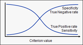
| ROC-AUC | Let’s first understand what is ROC (Receiver operating characteristic) curve. If we look at the confusion matrix, we observe that for a probabilistic model, we get different value for each metric.
Hence, for each sensitivity, we get a different specificity. The two vary as follows:
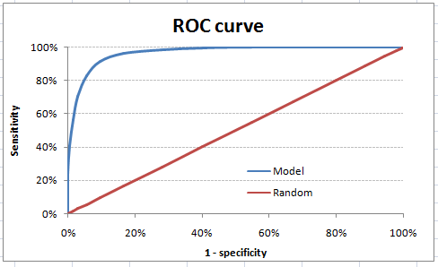
The ROC curve is the plot between sensitivity and (1- specificity). (1- specificity) is also known as false positive rate and sensitivity is also known as True Positive rate. Following is the ROC curve for the case in hand.
Let’s take an example of threshold = 0.5 (refer to confusion matrix). Here is the confusion matrix : As you can see, the sensitivity at this threshold is 99.6% and the (1-specificity) is ~60%. This coordinate becomes on point in our ROC curve. To bring this curve down to a single number, we find the area under this curve (AUC). Note that the area of entire square is 1*1 = 1. Hence, AUC itself is the ratio under the curve and the total area. |
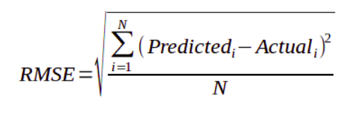
| Root Mean Squared Error (RMSE) | RMSE is a measure of the differences between values predicted by a model or an estimator and the values actually observed. It is the standard deviation of the residuals. Residuals are a measure of how far from the regression line data points are. The formula for RMSE is given by:
Here,
|
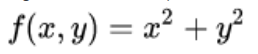
| Rotational Invariance | In mathematics, a function defined on an inner product space is said to have rotational invariance if its value does not change when arbitrary rotations are applied to its argument. For example, the function:
is invariant under rotations of the plane around the origin, because for a rotated set of coordinates through any angle θ. |
S
Word |
Description |
| Scala | Scala is a general purpose language that combines concepts of object-oriented and functional programming languages. Here are some key features of Scala
|
| Semi-Supervised Learning | Problems where you have a large amount of input data (X) and only some of the data, is labeled (Y) are called semi-supervised learning problems.
These problems sit in between both supervised and unsupervised learning. A good example is a photo archive where only some of the images are labeled, (e.g. dog, cat, person) and the majority are unlabeled. |
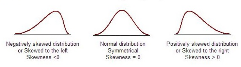
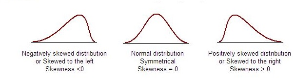
| Skewness |
Skewness is a measure of symmetry. A distribution, or data set, is symmetric if it looks the same to the left and right of the center point.
|
| SMOTE | It is a Synthetic Minority Over-Sampling Technique which is an approach to the construction of classifiers from imbalanced datasets is described. The idea behind this technique is that over-sampling the minority (abnormal) class and under-sampling the majority (normal) class can achieve better classifier performance (in ROC space) than only under-sampling the majority class. This is an over-sampling approach in which the minority class is over-sampled by creating “synthetic” examples rather than by over-sampling with replacement. To read further on SMOTE, refer here. |
| Spatial-Temporal Reasoning | Spatial-temporal reasoning is an area of artificial intelligence which draws from the fields of computer science, cognitive science, and cognitive psychology. Spatial-temporal reasoning is the ability to mentally move objects in space and time to solve multi-step problems. Three important things about Spatial-temporal reasoning are:
|
| Standard Deviation | Standard deviation signifies how dispersed is the data. It is the square root of the variance of underlying data. Standard deviation is calculated for a population. |
| Standardization | Standardization (or Z-score normalization) is the process where the features are rescaled so that they’ll have the properties of a standard normal distribution with μ=0 and σ=1, where μ is the mean (average) and σ is the standard deviation from the mean. Standard scores (also called z scores) of the samples are calculated as follows: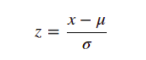 |
| Standard error | A standard error is the standard deviation of the sampling distribution of a statistic. The standard error is a statistical term that measures the accuracy of which a sample represents a population. In statistics, a sample mean deviates from the actual mean of a population this deviation is known as standard error. |
| Statistics | It is the study of the collection, analysis, interpretation, presentation, and organisation of data. |
| Stochastic Gradient Descent | Stochastic Gradient Descent is a type of gradient descent algorithm where we take a sample of data while computing the gradient. The update to the coefficients is performed for each training instance, rather than at the end of the batch of instances.
The learning can be much faster with stochastic gradient descent for very large training datasets and often one only need a small number of passes through the dataset to reach a good or good enough set of coefficients. |
| Supervised Learning | Supervised Learning algorithm consists of a target / outcome variable (or dependent variable) which is to be predicted from a given set of predictors (independent variables). Using these set of predictors, we generate a function that map inputs to desired outputs. Like: y= f(x)
Here, The goal is to approximate the mapping function so well that when you have new input data (x) that you can predict the output variables (Y) for that data. Examples of Supervised Learning algorithms: Regression, Decision Tree, Random Forest, KNN, Logistic Regression etc. |
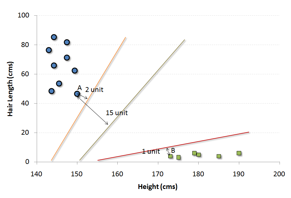
| SVM |
It is a classification method. In this algorithm, we plot each data item as a point in n-dimensional space (where n is the number of features you have) with the value of each feature being the value of a particular coordinate. For example, if we only have two features like Height and Hair length of an individual, we’d first plot these two variables in two-dimensional space where each point has two coordinates (these coordinates are known as Support Vectors) Now, we will find some line that splits the data between the two differently classified groups of data. This will be the line such that the distances from the closest point in each of the two groups will be farthest away.
|
T
Word |
Description |
| TensorFlow | TensorFlow, developed by the Google Brain team, is an open source software library. It is used for building machine learning models for range of tasks in data science, mainly used for machine learning applications such as building neural networks. TensorFlow can also be used for non- machine learning tasks that require numerical computation. |
| Tokenization | Tokenization is the process of splitting a text string into units called tokens. The tokens may be words or a group of words. It is a crucial step in Natural Language Processing. |
| Torch | Torch is an open source machine learning library, based on the Lua programming language. It provides a wide range of algorithms for deep learning. |
| Transfer Learning | Transfer learning refers to applying a pre-trained model on a new dataset. A pre-trained model is a model created by someone to solve a problem. This model can be applied to solve a similar problem with similar data.
Here you can check some of the most widely used pre-trained models. |
| True Negative | These are the points which are actually false and we have predicted them false. For example, consider an example where we have to predict whether the loan will be approved or not. Y represents that loan will be approved, whereas N represents that loan will not be approved. So, here the True negative will be the number of classes which are actually N and we have predicted them N as well. |
| True Positive | These are the points which are actually true and we have predicted them true. For example, consider an example where we have to predict whether the loan will be approved or not. Y represents that loan will be approved, whereas N represents that loan will not be approved. So, here the True positive will be the number of classes which are actually Y and we have predicted them Y as well. |
| Type I error | The decision to reject the null hypothesis could be incorrect, it is known as Type I error.
|
| Type II error | The decision to retain the null hypothesis could be incorrect, it is know as Type II error.
|
| T-Test | T-test is used to compare two population by finding the difference of their population means. For more, refer here. |
U
Word |
Description |
| Underfitting | Underfitting occurs when a statistical model or machine learning algorithm cannot capture the underlying trend of the data. It refers to a model that can neither model on the training data nor generalize to new data. An underfit model is not a suitable model as it will have poor performance on the training data. |
| Univariate Analysis | Univariate analysis is comparing and analyzing the dependency of a single predictor and a response variable |
| Unsupervised Learning | In Unsupervised Learning algorithm, we do not have any target or outcome variable to predict/estimate. The goal of unsupervised learning is to model the underlying structure or distribution in the data in order to learn more about the data or segment into different groups based on their attributes.Examples of Unsupervised Learning algorithm: Apriori algorithm, K-means. |
V
Word |
Description |
| Variance |
Variance is used to measure the spread of given set of numbers and calculated by the average of squared distances from the mean Let’s take an example, suppose the set of numbers we have is (600, 470, 170, 430, 300) |
Z
Word |
Description |
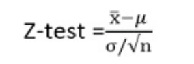
| Z-test | Z-test determines to what extent a data point is away from the mean of the data set, in standard deviation. For example:
Principal at a certain school claims that the students in his school are above average intelligence. A random sample of thirty students has a mean IQ score of 112. The mean population IQ is 100 with a standard deviation of 15. Is there sufficient evidence to support the principal’s claim? So we can make use of z-test to test the claims made by the principal. Steps to perform z-test:
Here,
If the test statistic is greater than the z-score of rejection area, reject the null hypothesis. If it’s less than that z-score, you cannot reject the null hypothesis. To get a better understanding of the topic, refer here. |
| Zookeeper | ZooKeeper is a software project of the Apache Software Foundation. It is an open source file application program interface (API) that allows distributed processes in large systems to synchronize with each other so that all clients making requests receive consistent data.
|