Case Study For Freshers (Level : Medium) – Call Center Optimization

Introduction

Last week, I introduced you to a classic problem of operational analytics. If you didn’t get a chance to check it, you can do it right here.

I had drafted it mainly for freshers who lack confidence in solving case studies. And, this becomes one of the key reason for their rejection in job interviews. Now, if you are still reading this, I take it that you ready to walk the next level with me!

I made the first level simple to understand to get you wanting to go to the next. It just required a logical understanding of how things happen in a call center.

However, that was an over simplified version of what actually happens in a call center. In this article, I will take a step forward and talk about a more real life case in a call center optimization problem. I believe it to be more helpful for R users as I’ve demonstrated the codes in R. However, even if you don’t know R, you can still work your way out in Excel.

Make sure you check out the ‘Ace Data Science Interviews‘ course for multiple such case studies. We have put together a very comprehensive course to help you successfully land your first data science job – don’t miss it!

We assumed multiple things in the previous case study. Some of which were:

1. All the calls come at the same time. In real case this will never happen.
2. The time taken by a caller to handle a customer is accurately predicted.

Let’s ease out the first assumption to make the case study more realistic.

Business Case (Level : Medium)

Assume, you are setting up a call center for a mid-sized E-Commerce firm. You have been asked to find the total strength of callers required for this requirement. This requirement will be outsourced to a call center which guarantees availability of caller for 24 hours with the exact same efficiency.

Using this efficiency, you have also estimated the time of each call from the customer and the duration of these calls. This estimation is based on your market research and prediction through customer behavior in past. You can assume that this prediction is accurate. Now, you need to estimate the following:

1. What is the minimum number of callers required if you need to ensure that no customer waits to reach out to the representative (Zero waiting time)?
2. What is the minimum number of callers required if you need to ensure that no customer waits for more than 30 minutes (Max. 30 minutes waiting time)?

Data you need to deal with

The data provided to you is of 10k calls which are made in a day. You can download the data here. The data looks something like this :

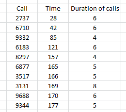
Here are few things you should consider:

1. The duration of calls is in “Minutes”.
2. Time is the time (in minutes) from 00:00 midnight.
3. Call represents the ID of the customer.
4. Assume that every caller has same efficiency and takes equal duration of calls  as given in data.
5. Also, you should assume that there were no breaks taken by the caller. And, individual caller is available for entire 24 hours. Note that the data is only for a single day (1440 minutes).

Let’s find the Solution

Explore Data

As always I say, it’s essential to explore and analyze data distribution at first. So, here is the distribution of call duration in the data:

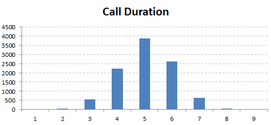
As you can observe most of the calls end up (call duration) between 3-7 minutes with a peak at 5 minutes. Let’s get to the next variable.

Here is the distribution of Call Timing :

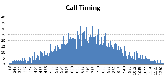
To me, it also looks normally distributed i.e. it follows a similar shape like previous graph. We see maximum calls arrive between 9 am to 4 pm with a peak at 12 noon.

We are done with exploring data. Now, we’ll get to the solution.

Solution

Let us start with a very simple solution. If we ignore the time when the calls were made, the sum of all call duration comes out to be 50635 minutes.

Available time for a caller (24*60) = 1440 minutes

Number of callers required =  (50635/ 1440) = 35.14

So we need approx. 36 callers if we had the choice to call back the customer whenever our caller is free. So, during interviews, when you don’t get much time but need an intuitive solution, such kind of assumptions work well! But the real life is not that simple. Here we need to account for the time at which customer called the call center.

Therefore, for the actual solution, you will need to simulate for every customer – caller combination. I am doing it in R, you can use any tool such as excel, python to accomplish this. Here is a simple R code:

#set working directory
> setwd("C:\\Tavs\\CC")

#Read data
> data <- read.csv("Case_Level2.csv")
> summary(data)

#Create a matrix where we will store the maximum waiting time for each value of the number of callers
> caller_opt <- matrix(0,100,2)

#Run loop for every number of callers possible. Here we have taken the range from 1 to 100
> for (number_of_callers in (1:100)){
               #Initialize the available time for each caller
               caller <- rep(0,number_of_callers)

               #Index will be used to refer a caller
               index <- 1:number_of_callers

               #Here we store the difference of each callers availability from the time when                the call was made
               caller_diff <- rep(0,number_of_callers)

               #We add two columns to the table : Caller assigned to the customer & Wait time                for the customer
               data$assigned <- 1
               data$waittime <- 0
               for (i in 1:length(data$Call))
               {
                    caller_diff <- data$Time[i] - caller
                    best_caller_diff <- max(caller_diff)
                    index1 <- index[min(index[caller_diff == best_caller_diff])]
                    data$assigned[i] <-  index1
                    data$waittime[i] <- max(-best_caller_diff,0)
                    caller[index1] <- caller[index1] + data$Duration.of.calls[i]
                }
                caller_opt[number_of_callers,1] = number_of_callers
                caller_opt[number_of_callers,2] = max(data$waittime)
                print(caller_opt[number_of_callers,])
}

Final Results

Here is what we get as the result:

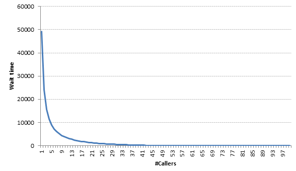
As you can observe from the graph that deciding the right number of callers is immensely important. Missing the number by just 10% can also increase the wait time for a customer significantly. In our case if we keep 4 call center reps less (~44), the maximum wait time for a customer becomes 87 minutes, which is something no company will ever want.

Therefore,

1. Answer 1 is 48 i.e. 48 callers are required to make sure we have no waiting time.
2. Answer 2 is 47 which gives a maximum wait time of 21 minutes i.e. we need minimum of 47 callers to ensure that no caller wait for more than 30 mins (max wait time is 30 mins).

End Notes

We have still managed to keep the case study simple enough by even varying the time of calling. However, two big assumptions still there are:

1. All Reps have the same efficiency
2. There is no rest time for the Reps.

Beyond these two assumption, we haven’t touched how to make predictions for call duration and call time. But this case study will give you a good feel of how to simulate an entire environment in such an operation intensive function. In future case studies, we will start relaxing these assumptions as well, making to simulation even more closer to reality.

Did you like reading this article ? Can you think of other checks to make this case study mimicking the actual call center in a better way? Do share your experience / suggestions in the comments section below.

You can test your skills and knowledge. Check out Live Competitions and compete with best Data Scientists from all over the world.

Tavish Srivastava

Tavish Srivastava, co-founder and Chief Strategy Officer of Analytics Vidhya, is an IIT Madras graduate and a passionate data-science professional with 8+ years of diverse experience in markets including the US, India and Singapore, domains including Digital Acquisitions, Customer Servicing and Customer Management, and industry including Retail Banking, Credit Cards and Insurance. He is fascinated by the idea of artificial intelligence inspired by human intelligence and enjoys every discussion, theory or even movie related to this idea.