Queuing theory Definition, Applications and Examples

Introduction

Queuing Theory, as the name suggests, is a study of long waiting lines done to predict queue lengths and waiting time. It’s a popular theory used largely in the field of operational, retail analytics. In my previous articles, I’ve already discussed the basic intuition behind this concept with beginner and  intermediate level case studies.

This is the last article of this series. Hence, make sure you’ve gone through the previous levels (beginner and intermediate).

Until now, we solved cases where volume of incoming calls and duration of call was known before hand. In real world, this is not the case. In real world, we need to assume a distribution for arrival rate and service rate and act accordingly. I wish things were less complicated! Let’s understand these terms:

Arrival rate is simply a result of customer demand and companies don’t have control on these. Service rate, on the other hand, largely depends on how many caller representative are available to service, what is their performance and how optimized is their schedule.

In this article, I will bring you closer to actual operations analytics using Queuing theory. We will also address few questions which we answered in a simplistic manner in previous articles.

What is Queuing Theory ?

As discussed above, queuing theory is a study of long waiting lines done to estimate queue lengths and waiting time. It uses probabilistic methods to make predictions used in the field of operational research, computer science, telecommunications, traffic engineering etc.

Queuing theory was first implemented in the beginning of 20th century to solve telephone calls congestion problems. Hence, it isn’t any newly discovered concept. Today, this concept is being heavily used by companies such as Vodafone, Airtel, Walmart, AT&T, Verizon and many more to prepare themselves for future traffic before hand.

Let’s dig into this theory now. We’ll now understand an important concept of queuing theory known as Kendall’s notation & Little Theorem.

How Queuing Theory Works?

Queuing theory, also known as queueing theory or waiting line theory, is the mathematical study of waiting lines. It delves into how they form, function, and potentially malfunction. By analyzing various aspects of a queue, queuing theory helps design efficient, cost-effective systems and provide good customer service.

Here’s a breakdown of how queuing theory works:

Key components:

• Customers: These can be people, objects, or even data packets waiting for service.
• Servers: These are the service resources, like cashiers, machines, or network channels.
• Queue discipline: This defines how customers are served, like first-in-first-out (FIFO), last-in-first-out (LIFO), or priority-based.
• Arrival process: This describes how customers arrive at the queue, like randomly or at specific intervals.
• Service process: This describes how service is provided, including its duration and variability.

What queuing theory analyzes:

• Average waiting time: How long customers typically wait in line.
• Queue length: The average number of customers in the queue.
• Server utilization: How busy the servers are on average.
• Probability of waiting: The likelihood of a customer arriving and waiting.

Applications of Queuing Theory:

Queuing theory is used in various fields to improve system performance and customer satisfaction. Here are some examples:

• Retail: Optimizing the number of cashiers needed during peak hours.
• Call centres: Determining the appropriate number of call centre agents to handle incoming calls efficiently.
• Traffic management: Designing intersections and traffic lights to reduce congestion.
• Computer networks: Managing data traffic and preventing bottlenecks.

Benefits:

• Reduced waiting times: By understanding queue dynamics, systems can be designed to minimize customer wait times.
• Improved resource allocation: Queuing theory helps allocate resources, like servers, efficiently, avoiding underutilization or overload.
• Cost optimization: Queuing theory can help find the most cost-effective solution by balancing waiting times and resource costs.
• Enhanced Capacity Planning: Queuing theory can forecast demand and plan for future capacity needs, ensuring systems handle expected workloads.
• Data-Driven Decision Making: Queuing theory insights provide a data-driven foundation for decisions on system design, staffing, and process improvements.

Kendall’s notation

This notation can be easily applied to cover a large number of simple queuing scenarios. This is a shorthand notation of the type A/B/C/D/E/F  where A, B, C, D, E,F describe the queue. Every letter has a meaning here. The various standard meanings associated with each of these letters are summarized below.

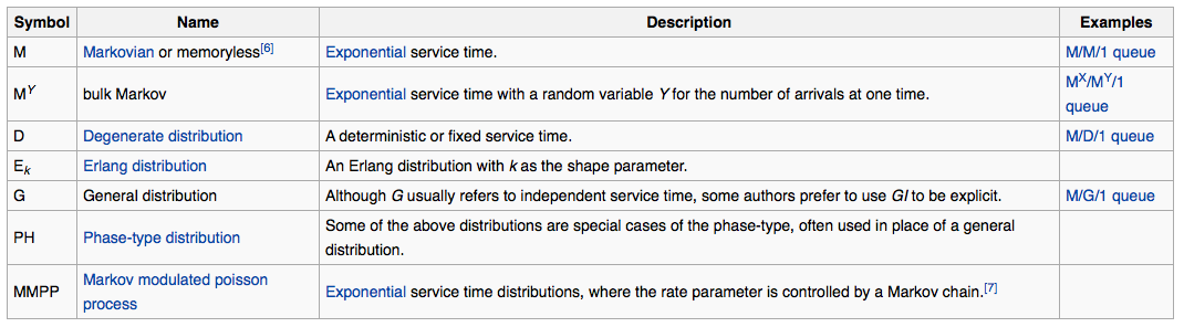
A is the Inter-arrival Time distribution . Here are the possible values it can take :

eory was first implemented in the beginning of 20th century to solve telephone calls congestion problems. Hence, it isn’t any newly discovered concept. Today, this concept is being heavily used by companies such as Vodafone,

B is the Service Time distribution. Here are the possible values it can take:

C gives the Number of Servers in the queue. It has to be a positive integer.

D gives the Maximum Number of jobs which are available in the system counting both those who are waiting and the ones in service. In case, if the number of jobs are not available, then the default value of infinity (∞) is assumed implying that the queue has an infinite number of waiting positions

E gives the number of arrival components. In general, we take this to be infinity (∞) as our system accepts any customer who comes in. However, in case of machine maintenance where we have fixed number of machines which requires maintenance, this is also a fixed positive integer.

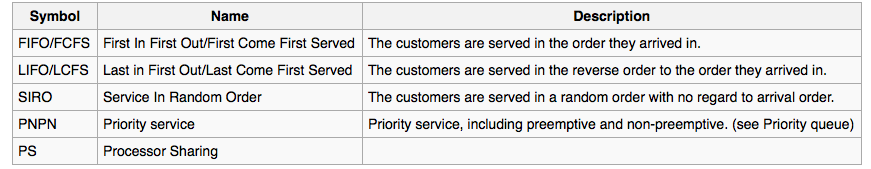
F represents the Queuing Discipline that is followed. The typical ones are First Come First Served (FCFS), Last Come First Served (LCFS), Service in Random Order (SIRO) etc.. If this is not given, then the default queuing discipline of FCFS is assumed. Possible values are :

The simplest member of queue model is M/M/1/∞/∞/FCFS.

This means that we have a single server; the service rate distribution is exponential; arrival rate distribution is poisson process; with infinite queue length allowed and anyone allowed in the system; finally its a first come first served model.

Parameters of Interest

A queuing model works with  multiple parameters. These parameters help us analyze the performance of our queuing model. Think of what all factors can we be interested in? Here are a few parameters which we would be interested for any queuing model:

1. Probability of no customer in the system
2. Probability of no queue in the system
3. Probability that the new customer will get a server directly as soon as he comes into the system
4. Probability that a new customer is not allowed in the system
5. Average length of the queue
6. Average population in the system
7. Average waiting time
8. Average time for a customer in the system

Little Theorem

It’s an interesting theorem. Let’s understand it using an example.

Consider a queue, incorporating principles from queuing theory, where a process with a mean arrival rate of λ actually enters the system. Let N be the mean number of jobs (customers) in the system, encompassing those both waiting and in service, and W represent the mean time spent by a job in the system, covering both the waiting and in-service durations. This perspective, rooted in queuing theory, helps analyze and optimize the efficiency of systems involving the flow of tasks or customers through a queue..

Little’s Result then states that these quantities will be related to each other as:

N= λW 

This theorem comes in very handy to derive the waiting time given the queue length of the system.

Parameters for 4 simplest series:

1. M/M/1/∞/∞

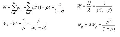
Here, N and Nq are the number of people in the system and in the queue respectively. Also W and Wq are the waiting time in the system and in the queue respectively. Rho is the ratio of arrival rate to service rate. Also the probabilities can be given as :

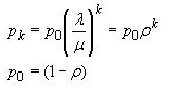
where, p0 is the probability of zero people in the system and pk is the probability of k people in the system.

2. M/M/1/∞/∞ Queue with Discouraged Arrivals :

This is one of the common distribution because the arrival rate goes down if the queue length increases. Imagine you went to Pizza hut for a pizza party in a food court. But the queue is too long. You would probably eat something else just because you expect high waiting time.

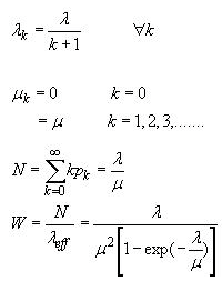
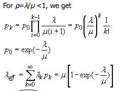
As you can see the arrival rate decreases with increasing k.

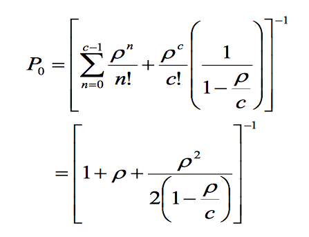
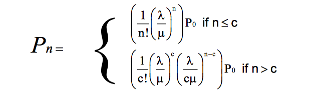
3. M/M/c/∞/∞

With c servers the equations become a lot more complex. Here are the expressions for such Markov distribution in arrival and service.

Case Study 1

Imagine, you work for a multi national bank. You have the responsibility of setting up the entire call center process. You are expected to tie up with a call centre and tell them the number of servers you require.

Setting up a call center to handle specific customer feature questions, there’s an influx of about 20 queries per hour. Each question takes roughly 15 minutes to resolve. Determine the number of servers or representatives needed to reduce the average waiting time to less than 30 seconds.

Solution

The given problem is a M/M/c type query with following parameters.

Lambda = 20
Mue = 4

Here is an R code that can find out the waiting time for each value of number of servers/reps.

> Lambda <- 20
> Mue <- 4

> Rho <- Lambda/Mue

#Create an empty matrix
> matrix <- matrix(0,10,2)
> matrix[,1] <- 1:10
#Create a function than can find the waiting time
> calculatewq <- function(c){
 P0inv <- Rho^c/(factorial(c)*(1-(Rho/c)))
 for (i in 1:c-1) {
 P0inv = P0inv + (Rho^i)/factorial(i)
 }
 P0 = 1/P0inv
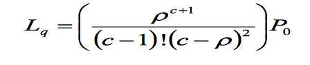
 Lq = (Rho^(c+1))*P0/(factorial(c-1)*(c-Rho)^2)
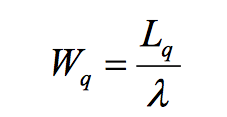
 Wq = 60*Lq/Lambda
 Ls <- Lq + Rho
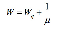
 Ws <- 60*Ls/Lambda
 #print(paste(Lq," is queue length and ",Wq," is the waiting time"))
 a <- cbind(Lq,Wq,Ls,Ws)
 return(a)
 }

#Now populate the matrix with each value of waiting time
> for (i in 1:10){
             matrix[i,2] <- calculatewq(i)[2]
             }

Here are the values we get for waiting time:

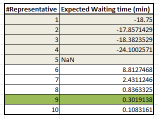
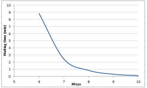
A negative value of waiting time means the value of the parameters is not feasible and we have an unstable system. Clearly with 9 Reps, our average waiting time comes down to 0.3 minutes.

Case Study 2

Let’s take a more complex example.

Imagine, you are the Operations officer of a Bank branch. Your branch can accommodate a maximum of 50 customers. How many tellers do you need if the number of customer coming in with a rate of 100 customer/hour and a teller resolves a query in 3 minutes ?

You need to make sure that you are able to accommodate more than 99.999% customers. This means only less than 0.001 % customer should go back without entering the branch because the brach already had 50 customers. Also make sure that the wait time is less than 30 seconds.

Solution

This is a “M/M/c/N = 50/∞” kind of queue system. Don’t worry about the queue length formulae for such complex system (directly use the one given in this code). Just focus on how we are able to find the probability of customer who leave without resolution in such finite queue length system.

Here is the R-code

> Lambda <- 100

> Mue <- 20
> Rho <- Lambda/Mue
> N <- 50

> matrix <- matrix(0,100,3)
> matrix[,1] <- 1:100
> calculatewq(6)

> calculatewq <- function(c){
 P0inv <- (Rho^c*(1-((Rho/c)^(N-c+1))))/(factorial(c)*(1-(Rho/c)))
 for (i in 1:c-1) {
 P0inv = P0inv + (Rho^i)/factorial(i)
 }
 P0 = 1/P0inv
 Lq = (Rho^(c+1))*(1-((Rho/c)^(N-c+1))-((N-c+1)*(1-(Rho/c))*((Rho/c)^(N-c))))*P0/(factorial(c-1)*(c-Rho)^2)
 Wq = 60*Lq/Lambda
 Ls <- Lq + Rho
 Ws <- 60*Ls/Lambda
 PN <- (Rho^N)*P0/(factorial(c)*c^(N-c))
 customer_serviced <- (1 - PN)*100
 #print(paste(Lq," is queue length and ",Wq," is the waiting time"))
 a <- cbind(Lq,Wq,Ls,Ws,customer_serviced)
 return(a)
 }

> for (i in 1:100){
 matrix[i,2] <- calculatewq(i)[2]
 matrix[i,3] <- calculatewq(i)[5]
 }

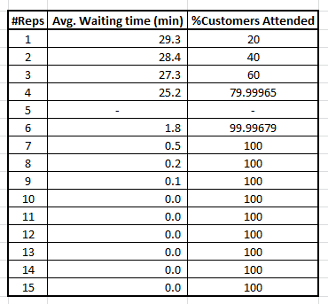
Clearly you need more 7 reps to satisfy both the constraints given in the problem where customers leaving

Conclusion

Queuing Theory, a branch of operations research, explores waiting lines’ behavior. By analyzing arrival rates, service times, and queue configurations, it optimizes systems. Applications span various fields, offering benefits like improved efficiency and resource utilization. Kendall’s notation categorizes queues, and Little’s Theorem aids in understanding queue dynamics, making Queuing Theory a valuable tool for managing complex processes.

Did you like reading this article ?  Do share your experience / suggestions in the comments section below.

You can test your skills and knowledge. Check out Live Competitions and compete with best Data Scientists from all over the world.

Tavish Srivastava

Tavish Srivastava, co-founder and Chief Strategy Officer of Analytics Vidhya, is an IIT Madras graduate and a passionate data-science professional with 8+ years of diverse experience in markets including the US, India and Singapore, domains including Digital Acquisitions, Customer Servicing and Customer Management, and industry including Retail Banking, Credit Cards and Insurance. He is fascinated by the idea of artificial intelligence inspired by human intelligence and enjoys every discussion, theory or even movie related to this idea.