Introduction
How easy would our life be if we took an already designed framework, executed it, and got the desired result? Minimum effort, maximum reward. Isn’t that what we strive for in any profession?
I feel fortunate to be part of our machine learning community, where even the top tech behemoths embrace open-source technology. Of course, it’s essential to understand and grasp concepts before implementing them, but it’s always helpful when top industry data scientists and researchers have laid the groundwork for you. In the realm of object detection, Yolo framework provide invaluable resources and tools for developers and researchers alike, further enriching our collective knowledge and capabilities.
This is especially true for deep learning domains like computer vision. Not everyone has the computational resources to build a DL model from scratch. That’s where predefined frameworks and pertained models come in handy. This article will look at one such framework for object detection – YOLO. It’s a swift and accurate YOLO framework, as we’ll see soon.
So far, in our series of posts detailing object detection (links below), we’ve seen the various algorithms used and how we can detect objects in an image and predict bounding boxes using algorithms of the R-CNN family. We have also looked at the implementation of Faster-RCNN in Python.
In part 3, we will learn what makes YOLO tick, why you should use it over other object detection algorithms, and the different techniques YOLO uses. Once we have understood the concept thoroughly, we will implement it in Python. It’s the ideal guide to gaining invaluable knowledge and applying it practically, hands-only.
I highly recommend going through the first two parts before diving into this guide:
- A Step-by-Step Introduction to the Basic Object Detection Algorithms (Part 1)
- A Practical Implementation of the Faster R-CNN Algorithm for Object Detection (Part 2)
Table of contents
What is YOLO Framework and Why is it Useful?
The R-CNN family of techniques we saw in Part 1 primarily uses regions to localize objects within the image. The network does not look at the entire picture, only the parts more likely to contain an object.
The YOLO framework (You Only Look Once), on the other hand, deals with object detection differently. It takes the entire image in a single instance and predicts the bounding box coordinates and class probabilities. The biggest advantage of using YOLO is its superb speed – it’s incredibly fast and can process 45 frames per second. YOLO also understands generalized object representation.
This is one of the best algorithms for object detection and has shown a performance that is comparatively similar to the R-CNN algorithms. In the upcoming sections, we will learn about different techniques used in YOLO algorithm. The following explanations are inspired by Andrew NG’s course on Object Detection, which helped me understand the workings of YOLO.
How does the YOLO Framework Function?
Now that we understand why YOLO is such a helpful framework. Let’s explore how it works. In this section, I have mentioned YOLO’s steps for detecting objects in a given image dataset.
- YOLO first takes an input image:
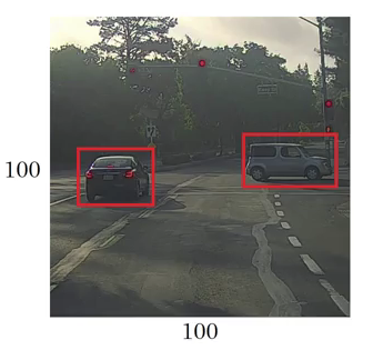
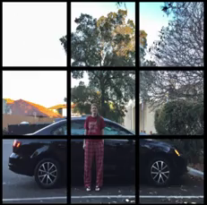
- The framework then divides the input image into grids (say a 3 X 3 grid):
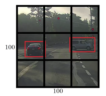
- Image classification and localization are applied on each grid. YOLO then predicts the bounding boxes and their corresponding class probabilities for objects (if any are found)
Pretty straightforward. Let’s break down each step to get a more granular understanding of what we just learned.
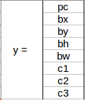
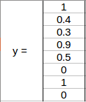
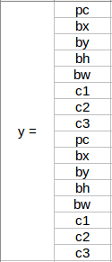
We need to pass the labeled data to the model to train it. Suppose we have divided the image into a grid of size 3 X 3, and there is a total of 3 classes that we want the objects to be classified into. The classes are Pedestrian, Car, and Motorcycle, respectively. So, for each grid cell, the label y will be an eight-dimensional vector:
Here,
- pc defines whether an object is present in the grid or not (it is the probability)
- bx, by, bh, bw specify the bounding box if there is an object
- c1, c2, c3 represent the classes. So, if the object is a car, c2 will be 1 and c1 & c3 will be 0, and so on
Let’s say we select the first grid from the above example:

Since there is no object in this grid, pc will be zero and the y label for this grid will be:
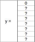
Here, ‘?’ means that it doesn’t matter what bx, by, bh, bw, c1, c2, and c3 contain as there is no object in the grid. Let’s take another grid in which we have a car (c2 = 1):

Before we write the y label for this grid, it’s essential first to understand how YOLO decides whether there is an object in the grid. In the above image, there are two objects (two cars), so YOLO framework will take the mid-point of these two objects, and these objects will be assigned to the grid that contains the mid-point of these objects. The y label for the center-left grid with the car will be:
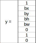
Since there is an object in this grid, pc will be equal to 1. bx, by, bh, and bw will be calculated relative to the particular grid cell we are dealing with since the car is the second class, c2 = 1 and c1 and c3 = 0. So, we will have an eight-dimensional output vector for each of the nine grids. This output will have a shape of 3 X 3 X 8.
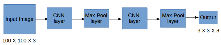
So now we have an input image and it’s corresponding target vector. Using the above example (input image – 100 X 100 X 3, output – 3 X 3 X 8), our model will be trained as follows:
We will run both forward and backward propagation to train our model. During testing, we pass an image to the model and run forward propagation until we get an output y. To keep things simple, I have explained this using a 3 X 3 grid here, but generally, in real-world scenarios, we take larger grids (perhaps 19 X 19).
Even if an object spans more than one grid, it will only be assigned to a single grid in which its mid-point is located. We can reduce the chances of multiple objects appearing in the same grid cell by increasing the number of grids (19 X 19, for example).
Also Read: How to Use Yolo v5 Object Detection Algorithm for Custom Object Detection?
How to Encode Bounding Boxes?
As I mentioned, bx, by, bh, and bw are calculated relative to the grid cell we are dealing with. Let’s understand this concept with an example. Consider the center-right grid, which contains a car:

So, bx, by, bh, and bw will be calculated relative to this grid only. The y label for this grid will be:
pc = 1 since there is an object in this grid, and since it is a car, c2 = 1. Now, let’s see how to decide bx, by, bh, and bw. In YOLO, the coordinates assigned to all the grids are:
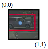
bx, by are the x and y coordinates of the midpoint of the object with respect to this grid. In this case, it will be (around) bx = 0.4 and by = 0.3:
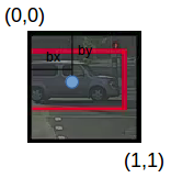
Bh is the ratio of the height of the bounding box (red box in the above example) to the height of the corresponding grid cell, which, in our case, is around 0.9. So, bh = 0.9. bw is the ratio of the bounding box’s width to the grid cell’s width. So, bw = 0.5 (approximately). The y label for this grid will be:
Notice here that bx and by will always range between 0 and 1, as the midpoint will always lie within the grid. Meanwhile, bh and bw can be more than 1 in case the dimensions of the bounding box are more than the dimensions of the grid.
The next section will examine more ideas that could potentially improve this algorithm’s performance.
Intersection over Union and Non-Max Suppression
Here’s some food for thought – how can we decide whether the predicted bounding box is giving us a good outcome (or a bad one)? This is where Intersection over Union comes into the picture. It calculates the intersection over the union of the actual bounding box and the predicted bounding box. Consider the actual and predicted bounding boxes for a car as shown below:
Here, the red box is the actual bounding box and the blue box is the predicted one. How can we decide whether it is a good prediction or not? IoU, or Intersection over Union, will calculate the intersection area over the union of these two boxes. That area will be:
IoU = Area of the intersection / Area of the union, i.e.
IoU = Area of the yellow box / Area of the green box
If IoU is greater than 0.5, we can say that the prediction is good enough. 0.5 is an arbitrary threshold we have taken here, but it can be changed according to your specific problem. Intuitively, the more you increase the threshold, the better the predictions.
One more technique can significantly improve the output of YOLO – Non-Max Suppression.
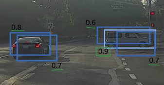
One of the most common problems with object detection algorithms is that rather than detecting an object just once, they might detect it multiple times. Consider the image below:
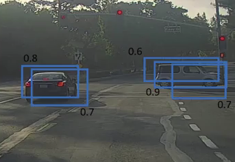
Here, the cars are identified more than once. The Non-Max Suppression technique cleans up this so we get only a single detection per object. Let’s see how this approach works.
1. It first looks at the probabilities associated with each detection and takes the largest one. In the above image, 0.9 is the highest probability, so the box with 0.9 probability will be selected first:
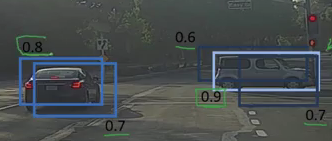
2. Now, it looks at all the other boxes in the image. The boxes that have high IoU with the current box are suppressed. So, the boxes with 0.6 and 0.7 probabilities will be suppressed in our example:
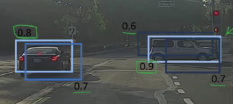
3. After the boxes have been suppressed, it selects the next box from all the boxes with the highest probability, which is 0.8 in our case:
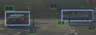
4. Again, it will look at the IoU of this box with the remaining boxes and compress the boxes with a high IoU:
5. We repeat these steps until all the boxes have either been selected or compressed and we get the final bounding boxes:
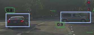
This is what Non-Max Suppression is all about. We are taking the boxes with maximum probability and suppressing the close-by boxes with non-max probabilities. Let’s quickly summarize the points that we’ve seen in this section about the Non-Max suppression algorithm:
- Discard all the boxes having probabilities less than or equal to a predefined threshold (say, 0.5)
- For the remaining boxes:
- Pick the box with the highest probability and take that as the output prediction
- Discard any other box that has IoU greater than the threshold with the output box from the above step
- Repeat step 2 until all the boxes are either taken as the output prediction or discarded
There is another method we can use to improve the performance of a YOLO algorithm – let’s check it out!
Anchor Boxes
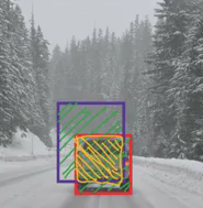
We have seen that each grid can only identify one object. But what if there are multiple objects in a single grid? That can so often be the case in reality. And that leads us to the concept of anchor boxes. Consider the following image divided into a 3 X 3 grid:
Remember how we assigned an object to a grid? We took the midpoint of the object and based on its location, assigned the object to the corresponding grid. In the above example, the midpoint of both objects lies in the same grid. This is how the actual bounding boxes for the objects will be:
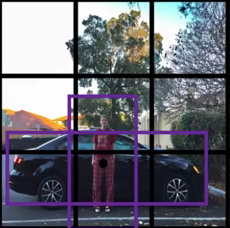
We will only be getting one of the two boxes for the car or the person. But if we use anchor boxes, we might be able to output both boxes! How do we go about doing this? First, we predefined two different shapes called anchor boxes or anchor box shapes. Now, instead of having one output, we will have two outputs for each grid. We can always increase the number of anchor boxes as well. I have taken two here to make the concept easy to understand:
This is how the y label for YOLO without anchor boxes looks like:
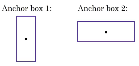
What would the ‘y’ label be if we had 2 anchor boxes? Please take a moment to ponder this before reading further. Got it? The y label will be:
The first 8 rows belong to anchor box 1, and the remaining 8 belong to anchor box 2. The objects are assigned to the anchor boxes based on the similarity of the bounding boxes and the anchor box shape. Since the shape of anchor box 1 is similar to the bounding box for the person, the latter will be assigned to anchor box 1, and the car will be transferred to anchor box 2. The output, in this case, instead of 3 X 3 X 8 (using a 3 X 3 grid and 3 classes), will be 3 X 3 X 16 (since we are using 2 anchors).
So, based on the number of anchors, two or more objects for each grid, based on the for each grid all the ideas we have covered so far are integrated into the YOLO framework.
Combining the Ideas
In this section, we will first see how a YOLO model is trained and how predictions can be made for a new and previously unseen image.
Training
The input for training our model will be images and their corresponding y labels. Let’s see an image and make its y label:
Consider the scenario where we are using a 3 X 3 grid with two anchors per grid, and there are 3 different object classes. So, the corresponding y labels will be 3 X 3 X 16. Suppose we use 5 anchor boxes per grid, and the number of classes has been increased to 5. So the target will be 3 X 3 X 10 X 5 = 3 X 3 X 50. This is how the training process is done – taking an image of a particular shape and mapping it with a 3 X 3 X 16 target (this may change as per the grid size, number of anchor boxes and the number of classes).
Testing
The new image will be divided into the same number of grids which we have chosen during the training period. For each grid, the model will predict an output of shape 3 X 3 X 16 (assuming this is the shape of the target during training time). The 16 values in this prediction will be in the same format as the training label’s. The first 8 values will correspond to anchor box 1, where the first value will be the probability of an object in that grid. Values 2-5 will be the bounding box coordinates for that object, and the last three values will tell us which class the object belongs to. The following 8 values will be for anchor box 2 and in the same format, i.e., first the probability, then the bounding box coordinates, and finally the classes.
Finally, the Non-Max Suppression technique will be applied to the predicted boxes to obtain a single prediction per object.
That brings us to the end of the theoretical aspect of understanding how the YOLO algorithm works, starting from training the model and then generating prediction boxes for the objects. Below are the exact dimensions and steps that the YOLO algorithm follows:
- Takes an input image of shape (608, 608, 3)
- Passes this image to a convolutional neural network (CNN), which returns a (19, 19, 5, 85) dimensional output
- The last two dimensions of the above output are flattened to get an output volume of (19, 19, 425):
- Here, each cell of a 19 X 19 grid returns 425 numbers
- 425 = 5 * 85, where 5 is the number of anchor boxes per grid
- 85 = 5 + 80, where 5 is (pc, bx, by, bh, bw) and 80 is the number of classes we want to detect
- Finally, we do the IoU and Non-Max Suppression to avoid selecting overlapping boxes
Evolution of YOLO Series in Object Detection Models
The YOLO series, comprising YOLOv1, YOLOv2, YOLOv3, YOLOv4, YOLOv5, YOLOv6, and YOLOv7, has significantly advanced the field of object detection with each iteration. The evolution of object detection models has seen significant advancements from YOLO to YOLOv8, each version addressing specific limitations while enhancing performance. The eContinuous improvements in model architecture, performance, and efficiency have marked the evolution: A Game-Changer in Object Detection.
YOLOv1 introduced fast R-CNN capabilities, revolutionizing object detection with its efficient recognition abilities. However, limitations emerged, notably in detecting smaller images within crowded scenes and unfamiliar shapes due to the single-object focus of its architecture. Additionally, the loss function’s uniform treatment of errors across different bounding box sizes led to inaccurate localizations.
YOLOv2: Enhancements for Better Performance
Enter YOLOv2, a refinement aimed at overcoming these drawbacks. Its adoption of Darknet-19 as a new architecture, alongside batch normalization, higher input resolution, and convolution layers using anchor boxes, marked significant progress. Batch normalization mitigated overfitting while improving performance, and higher input resolution enhanced accuracy, particularly for larger images. Convolution layers with anchor boxes simplified object detection, albeit with a slight accuracy tradeoff, offering improved recall for model enhancement. Dimensionality clustering further optimized performance, providing a balance between recall and precision through automated anchor box selection.
YOLOv3: Incremental Improvements
YOLOv3 continued improving with the introduction of Darknet-53, a larger, faster, and more accurate network architecture. The model refined bounding box prediction through logistic regression and enhanced class predictions with independent logistic classifiers, enabling more precise identification, especially in complex domains. Multiple predictions at different scales facilitated finer-grained semantic information extraction, yielding higher-quality output images.
YOLOv4: Optimal Speed and Accuracy
YOLOv4 marked a pinnacle in speed and accuracy, optimized for production systems with CSPDarknet53 as its backbone. Spatial Pyramid Pooling and PANet integration enhanced context feature extraction and parameter aggregation, respectively, without compromising speed. Data augmentation techniques like mosaic integration and optimal hyperparameter selection via genetic algorithms further improved model robustness and performance.
YOLOR: Unified Network for Multiple Tasks
YOLOR combined explicit and implicit knowledge approaches to create a robust architecture. It introduced prediction alignment, refinement, and canonical representation for improved performance across multiple tasks.
YOLOX: Exceeding Previous Versions
YOLOX surpassed earlier versions with an efficient decoupled head, robust data augmentation, an anchor-free system, and SimOTA for label assignment, resulting in improved performance and reduced training time.
YOLOv5: PyTorch Implementation
YOLOv5 was the first version implemented in PyTorch. It offers numerous model sizes and integrates a focus layer for reduced complexity and improved speed.
YOLOv6: Industrial Application Focus
YOLOv6 was tailored for industrial applications, featuring a hardware-friendly design, an efficient decoupled head, and a more effective training strategy, resulting in outstanding accuracy and speed.
YOLOv7: Setting New Standards
YOLOv7 set new standards with architectural reforms, including Extended Efficient Layer Aggregation Network (E-ELAN) integration and scalable architecture concatenation, alongside improvements in trainable bag-of-freebies, enhancing both speed and accuracy without increasing training costs.
Fpn (Feature Pyramid Network) integration in YOLOv7 further improved object detection performance, particularly in handling objects at different scales.
The YOLO versions, including YOLOv1 to YOLOv7, have been extensively discussed in research publications available on arXiv, contributing to the understanding and advancement of object detection algorithms.
Joseph Redmon, the creator of the YOLO algorithm, has played a crucial role in its development and popularization within the computer vision community.
Ground truth annotations, essential for training and evaluating object detection models, provide accurate labels for objects in images, enhancing model performance and generalization.
The COCO dataset, widely used in object detection research, provides a large-scale benchmark for training and evaluating models, ensuring robustness and comparability across different approaches.
Ali Farhadi, a prominent researcher in computer vision, has made significant contributions to the field, including work on detection and dataset creation.
The work YOLO framework series has revolutionized object detection with its continuous evolution, addressing challenges and pushing the boundaries of performance and efficiency. With each version, from YOLOv1 to YOLOv7, advancements in architecture, training strategies, and optimization techniques have propelled the field forward, setting new standards and inspiring further research and innovation.
Implementing YOLO Framework in Python
Time to fire up our Jupyter notebooks (or your preferred IDE) and finally implement our learning in the form of code! This is what we have been building up to so far, so let’s get the ball rolling.
The code we’llis section for implementing YOLO has been taken from Andrew NG’s GitHub repository on Deep Learning. You will also need to download the pre-trained weights required to run this code.
Let’s first define the functions that will help us choose the boxes above a certain threshold, find the IoU, and apply Non-Max Suppression on them. Before everything else, however, we’ll first import the required libraries:
import os
import matplotlib.pyplot as plt
from matplotlib.pyplot import imshow
import scipy.io
import scipy.misc
import numpy as np
import pandas as pd
import PIL
import tensorflow as tf
from skimage.transform import resize
from keras import backend as K
from keras.layers import Input, Lambda, Conv2D
from keras.models import load_model, Model
from yolo_utils import read_classes, read_anchors, generate_colors, preprocess_image, draw_boxes, scale_boxes
from yad2k.models.keras_yolo import yolo_head, yolo_boxes_to_corners, preprocess_true_boxes, yolo_loss, yolo_body

%matplotlib inline
Now, let’s create a function for filtering the boxes based on their probabilities and threshold:
def yolo_filter_boxes(box_confidence, boxes, box_class_probs, threshold = .6):
    box_scores = box_confidence*box_class_probs
    box_classes = K.argmax(box_scores,-1)
    box_class_scores = K.max(box_scores,-1)
    filtering_mask = box_class_scores>threshold
    scores = tf.boolean_mask(box_class_scores,filtering_mask)
    boxes = tf.boolean_mask(boxes,filtering_mask)
    classes = tf.boolean_mask(box_classes,filtering_mask)

    return scores, boxes, classes
Next, we will define a function to calculate the IoU between two boxes:
def iou(box1, box2):
    xi1 = max(box1[0],box2[0])
    yi1 = max(box1[1],box2[1])
    xi2 = min(box1[2],box2[2])
    yi2 = min(box1[3],box2[3])
    inter_area = (yi2-yi1)*(xi2-xi1)
    box1_area = (box1[3]-box1[1])*(box1[2]-box1[0])
    box2_area = (box2[3]-box2[1])*(box2[2]-box2[0])
    union_area = box1_area+box2_area-inter_area
    iou = inter_area/union_area

    return iou
Let’s define a function for Non-Max Suppression:
def yolo_non_max_suppression(scores, boxes, classes, max_boxes = 10, iou_threshold = 0.5):
    max_boxes_tensor = K.variable(max_boxes, dtype='int32')
    K.get_session().run(tf.variables_initializer([max_boxes_tensor]))
    nms_indices = tf.image.non_max_suppression(boxes,scores,max_boxes,iou_threshold)
    scores = K.gather(scores,nms_indices)
    boxes = K.gather(boxes,nms_indices)
    classes = K.gather(classes,nms_indices)

    return scores, boxes, classes
We now have the functions that will calculate the IoU and perform Non-Max Suppression. We get the output from the CNN of shape (19,19,5,85). So, we will create a random volume of shape (19,19,5,85) and then predict the bounding boxes:
yolo_outputs = (tf.random_normal([19, 19, 5, 1], mean=1, stddev=4, seed = 1),
                   tf.random_normal([19, 19, 5, 2], mean=1, stddev=4, seed = 1),
                   tf.random_normal([19, 19, 5, 2], mean=1, stddev=4, seed = 1),
                   tf.random_normal([19, 19, 5, 80], mean=1, stddev=4, seed = 1))
Finally, we will define a function which will take the outputs of a CNN as input and return the suppressed boxes:
def yolo_eval(yolo_outputs, image_shape = (720., 1280.), max_boxes=10, score_threshold=.6, iou_threshold=.5):
    box_confidence, box_xy, box_wh, box_class_probs = yolo_outputs
    boxes = yolo_boxes_to_corners(box_xy, box_wh)
    scores, boxes, classes = yolo_filter_boxes(box_confidence, boxes, box_class_probs, threshold = score_threshold)
    boxes = scale_boxes(boxes, image_shape)
    scores, boxes, classes = yolo_non_max_suppression(scores, boxes, classes, max_boxes, iou_threshold)

    return scores, boxes, classes
Let’s see how we can use the yolo_eval function to make predictions for a random volume which we created above:
scores, boxes, classes = yolo_eval(yolo_outputs)How does the outlook look?
with tf.Session() as test_b:
    print("scores[2] = " + str(scores[2].eval()))
    print("boxes[2] = " + str(boxes[2].eval()))
    print("classes[2] = " + str(classes[2].eval()))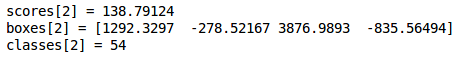
‘scores’ represents how likely the object will be present in the volume. ‘boxes’ return the (x1, y1, x2, y2) coordinates for the detected objects. ‘classes’ is the class of the identified object.
Now, let’s use a pre-trained YOLO algorithm on new images and see how it works:
sess = K.get_session()
class_names = read_classes("model_data/coco_classes.txt")
anchors = read_anchors("model_data/yolo_anchors.txt")

yolo_model = load_model("model_data/yolo.h5")
After loading the classes and the pre-trained model, let’s use the functions defined above to get the yolo_outputs.
yolo_outputs = yolo_head(yolo_model.output, anchors, len(class_names))Now, we will define a function to predict the bounding boxes and save the images with these bounding boxes included:
def predict(sess, image_file):
    image, image_data = preprocess_image("images/" + image_file, model_image_size = (608, 608))
    out_scores, out_boxes, out_classes = sess.run([scores, boxes, classes], feed_dict={yolo_model.input: image_data, K.learning_phase(): 0})

    print('Found {} boxes for {}'.format(len(out_boxes), image_file))

    # Generate colors for drawing bounding boxes.
    colors = generate_colors(class_names)

    # Draw bounding boxes on the image file
    draw_boxes(image, out_scores, out_boxes, out_classes, class_names, colors)

    # Save the predicted bounding box on the image
    image.save(os.path.join("out", image_file), quality=90)

    # Display the results in the notebook
    output_image = scipy.misc.imread(os.path.join("out", image_file))

    plt.figure(figsize=(12,12))
    imshow(output_image)

    return out_scores, out_boxes, out_classes
Next, we will read an image and make predictions using the predict function:
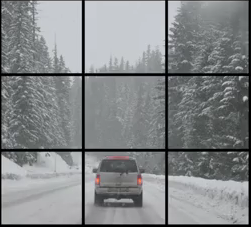
img = plt.imread('images/img.jpg')
image_shape = float(img.shape[0]), float(img.shape[1])
scores, boxes, classes = yolo_eval(yolo_outputs, image_shape)
Finally, let’s plot the predictions:
out_scores, out_boxes, out_classes = predict(sess, "img.jpg")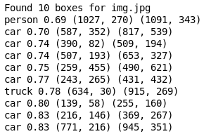
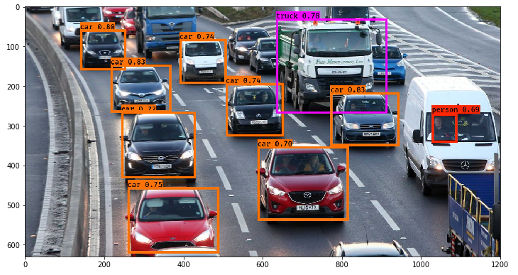
Not bad! I especially like that the model correctly picked up the person in the mini-van as well.
Conclusion
YOLO Framework (You Only Look Once) emerges as a groundbreaking framework in object detection, offering remarkable speed and accuracy. Its architecture, processing entire images in a single pass, sets it apart from traditional methods, making it ideal for real-time applications. The evolution of YOLO through versions like YOLOv1 to YOLOv7 showcases significant advancements, addressing limitations and enhancing performance with each iteration. Key features such as anchor boxes, intersection over union, and non-max suppression contribute to its effectiveness in detecting objects of various sizes and classes. Moreover, implementing Python provides a practical approach to understanding and utilizing this robust algorithm. With its widespread adoption across industries like surveillance, autonomous vehicles, and robotics, YOLO continues to shape the landscape of computer vision, offering researchers and practitioners a valuable tool for object detection tasks. From its YOLO Framework architecture to learning models and epochs, YOLO’s impact is undeniable, with benchmarks setting new standards for detection efficiency, particularly in handling small objects.
Here’s a summary of what we covered and implemented in this guide:
- YOLO Framework is a state-of-the-art object detection algorithm that is incredibly fast and accurate
- We send an input image to a CNN which outputs a 19 X 19 X 5 X 85 dimension volume.
- Here, the grid size is 19 X 19, each containing 5 boxes.
- We filter through all the boxes using Non-Max Suppression, keep only the accurate boxes, and also eliminate overlapping boxes
Frequently Asked Questions
Q1.What is the Yolo framework?
YOLO (You Only Look Once) is a real-time object detection framework that rapidly identifies objects in images or video streams. It employs a single neural network to simultaneously predict bounding boxes and class probabilities. YOLO’s strength lies in its efficiency, capable of processing images in real-time due to its single forward pass architecture. This makes it ideal for applications like surveillance, autonomous vehicles, and robotics. YOLO leverages GPUs for accelerated processing, making it highly efficient for real-time tasks.
Q2.Is Yolo a type of CNN?
Yes, YOLO is a convolutional neural network (CNN) type. It’s specifically designed for real-time object detection, unlike traditional CNNs that are primarily used for classification tasks like those seen in ImageNet challenges. YOLO utilizes convolutional layers for feature extraction and classification, but it differs in its architecture by directly predicting bounding boxes and class probabilities in a single pass, making it efficient for real-time applications.
Q3.What are YOLO Models Used For?
YOLO models are used for object detection tasks, serving as efficient object detectors. They employ classifiers and regression techniques to directly create bounding boxes and class probabilities through activation functions and feature maps; they extract relevant information from input images. Optimization methods enhance their accuracy and speed, making them valuable in applications requiring real-time object detection, such as surveillance, autonomous driving, and robotics
Q4.How Does YOLO Object Detection Work?
YOLO (You Only Look Once) object detection works by dividing an image into a grid and predicting bounding boxes and class probabilities for objects within each grid cell. Utilizing a deep convolutional neural network (CNN), typically implemented in the Darknet framework, YOLO extracts features and predicts bounding boxes directly. It’s efficient due to its single forward pass architecture, enabling real-time processing. Recent advancements like YOLOv4 and YOLOv5 have improved accuracy and speed. Unlike segmentation methods, YOLO does not rely on region proposals, resulting in faster inference. Metrics such as mAP (mean Average Precision) evaluate its performance.
Q5.What are the key differences between YOLOv2, YOLOv3 and YOLOv4?
The critical differences between YOLOv2, YOLOv3, and YOLOv4 lie in their architectures, performance, and features. YOLOv2 introduced the Darknet-19 architecture, improved anchor boxes, and multi-scale training, enhancing detection accuracy. YOLOv3 further refined detection performance with Darknet-53 architecture, feature pyramid network, and additional improvements in box prediction. YOLOv4, built upon YOLOv3, incorporated advancements like CSPNet, PANet, and improved training techniques, achieving superior detection accuracy and speed. While YOLOv4 introduced more robustness, YOLOv3 remains famous for its balance between accuracy and speed. Implementations vary with OpenCV, PyTorch, or other frameworks, each offering different arguments for efficiency and ease of use.
Pulkit Sharma
15 Feb, 2024
My research interests lies in the field of Machine Learning and Deep Learning. Possess an enthusiasm for learning new skills and technologies.


Thanks for article. How does YOLO compare with Faster-RCNN for detection of very small objects like scratches on metal surface? My observation was - RCNN lacks an elegant way to compute anchor sizes based on dataset... also I attempted changing scales,strides,box size results are bad. How do we custom train for YOLO?
Hi, YOLO is faster in comparison to Faster-RCNN. Their accuracies are comparatively similar. YOLO does not work pretty well for small objects. In order to improve its performance on smaller objects, you can try the following things:
- Increase the number of anchor boxes
- Decrease the threshold for IoU
This may give better results.Is this Yolo implemented on GPU based? How to training Yolo for customize object? Is are sany yolo code or tutorial using Tensorflow GPU base is available ? I only want to did detect vehicles. Please guide me.
Hi Hamza, Yes, I have trained this model on GPU. For customized training, you can pass your own dataset and the bounding boxes and train the model to get weights.
Hi PulKit, Very nicely explained article. In your Training paragraph , you have said that the output vector for 5 anchor boxes and 5 classes will be 3X3X25, shouldnt it be 3X3X50 instead , 50 comprising of [object(y/N)(1),coordinates of boundary box(4),5 classes(1 for each class) ] X no. of anchor boxes . i.e 10 X 5. = 50 Pls correct me if wrong
Hi Priya, That's correct. I have updated it in the article. Thanks for pointing it out
I can't find any zip file of pretrained weights for backend too. So, what should I do.
I followed the instructions as given but there are a lot of errors in classification. It is identifying objects but not correctly. Any reason why this might be happening?
Hi Arijeet, Can you share some of the results? You can try to train your own model as well instead of using the trained weights.
Hello Pulkit Sharma , How do you rate YOLO working for Face(face also being a type of object) detection, especially in video frames from surveillance feeds. ? Kindly also comment on the speed(real time performance) of this.What type of h/w platform would suit. ? How do you compare its performance with that of Voila Jones frame work (keeping human face as the object,in mind) regards, Thank you.
Hi Valli Kumar, I have not yet tested YOLO for detecting faces. For object detection it is faster than most of the other object detection techniques so, I hope it will also work good for face detection. I am currently working on the same project. First I will try different RNN techniques for face detection and then will try YOLO as well. Then only we can compare it with the other techniques. I will share the results as soon as I am done with this project.
Hi Pulkit, The article explains the concept with ease. Thanks for the nice article. I want to implement the YOLO v2 on a customized dataset. The input dimension is greater than the required size of YOLOv2(400x400 pixels). My doubt is should I resize the images and annotated them or is it fine to train the model with original annotations and resized images?
Hi Ganesh, If you are resizing the image, annotations should also be resized accordingly. If you use the original annotations, you will not get desired results.
how to train our own dataset with yolo v3
Hi Muhammed, You can refer to this article to learn how to train yolo on custom dataset.
I'm not able to load yolo.h5. When I so the kernel crashes. What do I do in this case?
Hi Shree, What is the configuration of your system? Does it have a GPU? If not, try to use Google colab which will give you access to free GPU.
Hi there I just wanted to get some advice in terms of YOLOv3. I am testing it to see how well it does in detecting strawberries in a field. As strawberries grow in clusters, it can be hard to distinguish them individually. Is there any advice you can give me in regard to improving results for such a problem, and any other deep learning object detection architectures I could try out. Thanks in advance.
Hi PULKIT, I load model using my own custom pre-train instead of yolo.h5. My model has only 2 classes. I run following your code and I got error because of "yolo_head" function in keras_yolo.py . the error look ===> Traceback (most recent call last): File "C:\Python36\Food-Diary_Project\YOLO_Food-Diary_new\YOLO_food_prediction_new.py", line 87, in yolo_outputs = yolo_head(yolo_model.output, anchors, len(class_names)) File "C:\Python36\Food-Diary_Project\YOLO_Food-Diary_new\yad2k\models\keras_yolo.py", line 109, in yolo_head conv_index = K.cast(conv_index, K.dtype(feats)) File "C:\Python36\lib\site-packages\keras\backend\tensorflow_backend.py", line 649, in dtype return x.dtype.base_dtype.name AttributeError: 'list' object has no attribute 'dtype' How can I solve this issue?
Did you fix it? I am getting same error
Hey, Can you tell me how to apply YoLo algorithm on video which is captured by webcam??
hi sharma, we are designing a project.We are making a combat unmanned aerial vehicle. In the real-time processing of the image taken from the camera, we use phython raspberry pi and opencv.how can we use the YOLO in this project.
How YOLO decide the mid point of those two object, and also it's confusing that mid point between those two objects or mid point of each object
Where to save the downloaded zip file having pre-trained weights.
Hi PULKIT, Thanks for the nice article. I have a question for you. You said : "In the above image, there are two objects (two cars), so YOLO will take the mid-point of these two objects and these objects will be assigned to the grid which contains the mid-point of these objects." My question : How does YOLO know (detect) that there is two objects before he can take the mid-point and assigne the object to the grid which contains the mid-point of these objects ?. Thank you in advance
Hi Pulkit, in IoU section, you said that box with IoU greater than 0.5 will be ignored in this case, isn't it inverse to what you just said?
Hi Ahsan, Firstly, we select the bounding box with the maximum probability. Now, we calculate the IoU of other bounding boxes with the box that we have selected. If this IoU is more, than we can infer that both the boxes are for the same object and can be removed. This is exactly what have been explained in the article as well.
Hii Pulkit sir I have two doubts kindly resolve it because i got same during andrew ng course 1.) You said that grid cell containing the midpoint of the object will be assigned positive and bounding boxes will be predicted but sir what i can see in images bounding boxes are spread to multiple gridcells depending upon the size of the object so how we predict bounding boxes in each grid cell which doesn't have midpoint because i think only one gridcell has the midpoint of object 2.) In non max supression you said that there will be multiple bounding boxes predictions but how ??
Hii this is a huge mess for me i am not understanding yolo my questions are still unaswered 1.) How yolo make bounding boxes for object bigger then it's grid cell 2. ) How confidence is calculated for that bigger box 3.) How multiple boxes are predicted Please help me out
Hello Pulkit, I am preparing my model using celeb dataset for gender recognition. Firstly I prepare my training dataset then model but during model I am getting error i.e Negative dimension size caused by subtracting 2 from 1 for 'MaxPool_32' (op: 'MaxPool') with input shapes: [?,50,1,16]. my code for model is-- model = Sequential() model.add(Convolution2D(16, 3, 3,input_shape=(50,50,1),border_mode='same',subsample=(1,1))) model.add(LeakyReLU(alpha=0.1)) model.add(MaxPooling2D(pool_size=(2, 2))) model.add(Convolution2D(32,3,3 ,border_mode='same')) model.add(LeakyReLU(alpha=0.1)) model.add(MaxPooling2D(pool_size=(2, 2),border_mode='valid')) model.add(Convolution2D(64,3,3 ,border_mode='same')) model.add(LeakyReLU(alpha=0.1)) model.add(MaxPooling2D(pool_size=(2, 2),border_mode='valid')) model.add(Convolution2D(128,3,3 ,border_mode='same')) model.add(LeakyReLU(alpha=0.1)) model.add(MaxPooling2D(pool_size=(2, 2),border_mode='valid')) model.add(Convolution2D(256,3,3 ,border_mode='same')) model.add(LeakyReLU(alpha=0.1)) model.add(MaxPooling2D(pool_size=(2, 2),border_mode='valid')) model.add(Convolution2D(512,3,3 ,border_mode='same')) model.add(LeakyReLU(alpha=0.1)) model.add(MaxPooling2D(pool_size=(2, 2),border_mode='valid')) model.add(Convolution2D(1024,3,3 ,border_mode='same')) model.add(LeakyReLU(alpha=0.1)) model.add(Convolution2D(1024,3,3 ,border_mode='same')) model.add(LeakyReLU(alpha=0.1)) model.add(Convolution2D(1024,3,3 ,border_mode='same')) model.add(LeakyReLU(alpha=0.1)) model.add(Flatten()) model.add(Dense(256)) model.add(Dense(4096)) model.add(LeakyReLU(alpha=0.1)) model.add(Dense(1470)) model.compile(loss='sparse_categorical_crossentropy', optimizer='adam', metrics=['accuracy']) model.fit(X, y, batch_size=32, nb_epoch=10, validation_split=0.1)
Hi Kunal, You can either try to increase the size of the images or reduce the max pool size.
can we detect the only person using this technique
Hi Kalpesh, Yes! You can. For this case, you first have to train your own model. So, you can train the model for detecting just the persons in the image. To do so, you can just give the true labels (bounding boxes for object detection case) for the persons in the image and train the model. Once the model is trained, you can test the model by predicting on new images and the model should generate the bounding boxes for all the persons in those new images.
Hi. When I want to run your code for an image, I got this error message: InvalidArgumentError: Dimensions must be equal, but are 2 and 80 for 'mul_7' (op: 'Mul') with input shapes: [?,?,?,5,2], [?,?,?,5,80]. How could I resolve it? Thanks
So, at what point is the grid created, meaning, if I have an image of 256x256, and I want to apply a 10x10 grid, where exactly does that happen?
Thanks for the explanation Pulkit. Can you please suggest me how to train customized yolo model on Google Colab. I have bounding box coordinates as well as annotations for the objects. How to feed our own data to the algorithm. P.S: I am using Google Colab.
This site is really interesting and easy to understand.
What is yolo_anchors.txt file ? Please tell me sample input for this file
Hi Guys, Thanks for Yolo. I have a requirement to run multiple instances like cam1, cam2... And also how to stop/quit the running instances explicitly means on demand based on time. Could you please help? I searched many sites but was not able to find a solution. Thanks inadvance.