Hands-On Introduction to creditR: An Amazing R Package to Enhance Credit Risk Scoring and Validation

Introduction

Machine learning is disrupting multiple and diverse industries right now. One of the biggest industries to be impacted – finance.

Functions like fraud detection, customer segmentation, employee or client retention are primary machine learning targets. The one we are going to focus on in this article is called credit risk scoring.

Credit scoring is a statistical analysis performed by lenders and financial institutions to access a person’s creditworthiness. Lenders use credit scoring, among other things, to decide on whether to extend or deny credit. – Investopedia

Machine learning algorithms are often developed as challenger models because this is a field where regulatory requirements need to be met. This got me thinking – how can I make things easier for professionals working in the field?

Out of that came the creditR package! It allows you to easily create your base models for credit risk scoring before machine learning applications. Additionally, the package also contains some functions that can be used to validate these processes.

The package aims to facilitate the applications of the methods of variable analysis, variable selection, model development, model calibration, rating scale development and model validation. Through the functions defined, these methodologies can be applied quickly on all modeling data or a specific variable.

In this article, we will first understand the nuts and bolts of the creditR package. We’ll then get our hands dirty in R by deep diving into a comprehensive example using creditR.

The package was issued for the use of credit risk professionals. Basic level knowledge about credit risk scoring methodologies is required for use of the package.

Table of Contents

1. Why should you use creditR?
2. Getting Started with creditR
3. A List of Functions inside creditR
4. An Application of the creditR Package

Why should you use creditR?

Perceptions of credit risk modeling are rapidly transforming as the demand for machine learning models in the field increases. However, many regulators are still very cautious about transitioning into machine learning techniques. Therefore, a possible speculation might be that during this transformation phase, machine learning algorithms will proceed along with the traditional methods.

Trust may be achieved on the part of the regulators once it is established that machine learning algorithms, while challenging the conventions of the field,  are also producing more robust results than the traditional methods. Moreover, the new methods of interpreting machine learning algorithms may help to create a more transparent process.

The creditR package offers both possibilities for automating the use of traditional methods and also for the validation of traditional and machine learning models.

Getting Started with creditR

In order to install the creditR package, you should have the devtools package installed. The devtools package can be installed by running the following code:

install.packages("devtools", dependencies = TRUE)

The creditR package can be installed using the “install_github” function found in the devtools package:

library(devtools)
devtools::install_github("ayhandis/creditR")
library(creditR)

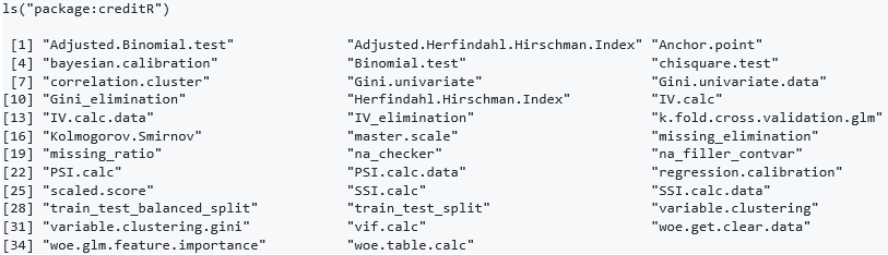
A List of Functions inside creditR

The functions available under the package are listed below.

ls("package:creditR")

Output:

An Application of the creditR Package

We’ve aprsed through the theory aspect. Now let’s get our hands dirty in R!

An example application of creditR is shared below in a study of how some common steps in credit risk scoring are carried out using the functions provided in the package.

Real-world practices were taken into consideration in the preparation of this example.

The general application is structured under two main headings as modeling and model validation, and the details as to what the corresponding code does can be seen in the comment lines.

Only important outputs have been shared in this article.

This R script is designed to make the creditR package easier to understand. Obtaining a high accuracy model is not within the scope of this study.

# Attaching the library
library(creditR)

#Model data and data structure
data("germancredit")
str(germancredit)

#Preparing a sample data set
sample_data <- germancredit[,c("duration.in.month","credit.amount","installment.rate.in.percentage.of.disposable.income", "age.in.years","creditability")]

#Converting the ‘Creditability’ (default flag) variable into numeric type
sample_data$creditability <- ifelse(sample_data$creditability == "bad",1,0)

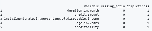
#Calculating the missing ratios
missing_ratio(sample_data)

Output:

#Splitting the data into train and test sets
traintest <- train_test_split(sample_data,123,0.70)
train <- traintest$train
test <- traintest$test

WOE transformation is a method which transforms the variable into a categorical variable through its relationship with the target variable. The following “woerules” object contains the WOE rules.

With the help of the woe.binning.deploy function, the rules were run on the data set. The variables we needed are assigned to the “train_woe” object with the help of the “woe.get.clear.data” function.

#Applying WOE transformation on the variables
woerules <- woe.binning(df = train,target.var = "creditability",pred.var = train,event.class = 1)
train_woe <- woe.binning.deploy(train, woerules, add.woe.or.dum.var='woe')

#Creating a dataset with the transformed variables and default flag
train_woe <- woe.get.clear.data(train_woe,default_flag = "creditability",prefix = "woe")

#Applying the WOE rules used on the train data to the test data
test_woe <- woe.binning.deploy(test, woerules, add.woe.or.dum.var='woe')
test_woe <- woe.get.clear.data(test_woe,default_flag = "creditability",prefix = "woe")

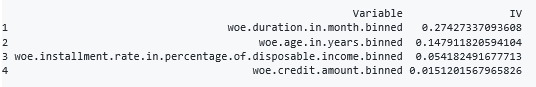
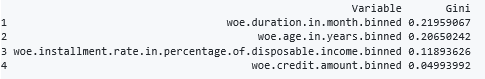
Information value and univariate gini can be used as variable selection methods. Generally, a threshold value of 0.30 is used for IV and 0.10 is used for univariate Gini.

#Performing the IV and Gini calculations for the whole data set
IV.calc.data(train_woe,"creditability")

Output:

Gini.univariate.data(train_woe,"creditability")

Output:

#Creating a new dataset by Gini elimination. IV elimination is also possible
eliminated_data <- Gini_elimination(train_woe,"creditability",0.10)
str(eliminated_data)

Output:

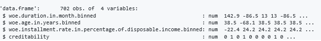
There are too many variables in real life to manage with correlation matrices. Hence, clustering is performed to determine variables with similar characteristics. This particular example of clustering does not make sense because of the small number of variables, but the method in general can be very useful in data sets with a large amounts of variables.

#A demonstration of the functions useful in performing Clustering
clustering_data <- variable.clustering(eliminated_data,"creditability", 2)
clustering_data

Output:

# Returns the data for variables that have the maximum gini value in the dataset
selected_data <- variable.clustering.gini(eliminated_data,"creditability", 2)

In some cases, average correlations of clusters are important because the number of clusters may not be set correctly. Therefore, if the cluster has a high average correlation, it should be examined in detail. The correlation value, which is only one variable in cluster 1, is NaN.

correlation.cluster(eliminated_data,clustering_data,variables = "variable",clusters = "Group")

Output:

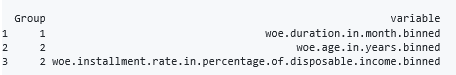
A model was formed with the variables included in the data set. When the variables are examined by the model summary, it seems that the variables are meaningful. Then, with the help of the “woe.glm.feature.importance” function, the weights of the variables are calculated. In fact, weights are calculated on the basis of the effect of a single unit change on the probability.

#Creating a logistic regression model of the data
model= glm(formula = creditability ~ ., family = binomial(link = "logit"),  data = eliminated_data)
summary(model)

Output:

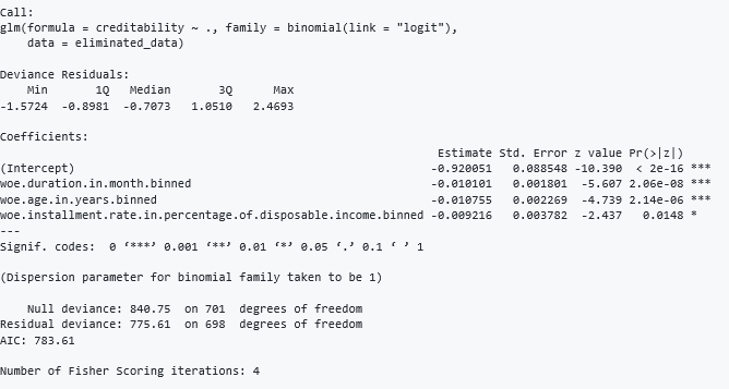
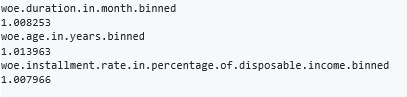
#Calculating variable weights
woe.glm.feature.importance(eliminated_data,model,"creditability")

Output:

#Generating the PD values for the train and test data
ms_train_data <- cbind(eliminated_data,model$fitted.values)
ms_test_data <- cbind(test_woe[,colnames(eliminated_data)], predict(model,type = "response", newdata = test_woe))
colnames(ms_train_data) <- c("woe.duration.in.month.binned","woe.age.in.years.binned","woe.installment.rate.in.percentage.of.disposable.income.binned","creditability","PD")
colnames(ms_test_data) <- c("woe.duration.in.month.binned","woe.age.in.years.binned","woe.installment.rate.in.percentage.of.disposable.income.binned","creditability","PD")

In real life, institutions use rating scales instead of continuous PD values. Due to some regulatory issues or to adapt to changing market/portfolio conditions, the models are calibrated to different central tendencies.

Regression and Bayesian calibration methods are included in the package. The numerical function that can perform calibration by embedding in the enterprise system can be obtained as output with the help of the “calibration object$calibration_formula” code.

#An example application of the Regression calibration method. The model is calibrated to the test_woe data
regression_calibration <- regression.calibration(model,test_woe,"creditability")
regression_calibration$calibration_data
regression_calibration$calibration_model
regression_calibration$calibration_formula

Output:

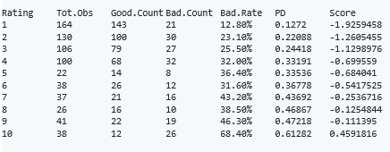
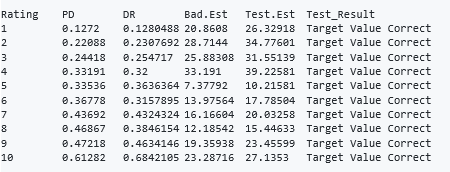
The Bayesian calibration method is applied over the rating scale. We can easily create the rating scale with the help of the “master.scale” function. However, in real life, rating scales can only be created after many trials.

The summary is added to the output. Details can be seen by running the R script. In addition, the example is only aimed to introduce the function within the scope of this study, hence, the PD values do not increase monotonically.

#Creating a master scale
master_scale <- master.scale(ms_train_data,"creditability","PD")
master_scale

Output:

In order to apply Bayesian calibration, the score variable is created in the data set. Then the rating scale is calibrated to 5% central tendency.

#Calibrating the master scale and the modeling data to the default rate of 5% using the bayesian calibration method
ms_train_data$Score = log(ms_train_data$PD/(1-ms_train_data$PD)) 
ms_test_data$Score = log(ms_test_data$PD/(1-ms_test_data$PD)) 
bayesian_method <- bayesian.calibration(data = master_scale,average_score ="Score",total_observations = "Total.Observations",PD = "PD",central_tendency = 0.05,calibration_data = ms_train_data,calibration_data_score ="Score")

#After calibration, the information and data related to the calibration process can be obtained as follows
bayesian_method$Calibration.model
bayesian_method$Calibration.formula

Output:

In real life applications, it is difficult to understand the concept of probability for employees who are not familiar with risk management. Therefore, there is a need to create a scaled score. This can be done simply by using the “scaled.score” function.

#The Scaled score can be created using the following function
scaled.score(bayesian_method$calibration_data, "calibrated_pd", 3000, 15)

After the modeling phase, the model validation is performed to validate different expectations such as the accuracy and stability of the model. In real life, a qualitative validation process is also applied.

Note: Model calibration is performed for illustration only. Model validation tests proceed through the original master scale as follows.

In the models created by logistic regression, the problem of multicollinearity should be taken into consideration. Although different threshold values are used, vif values greater than 5 indicate this problem.

#Calculating the Vif values of the variables.
vif.calc(model)

Output:

Generally, acceptable lower limit is 0.40 for Gini coefficient. However, this may vary according to model types.

#Calculating the Gini for the model
Gini(model$fitted.values,ms_train_data$creditability)

Output:

0.3577422

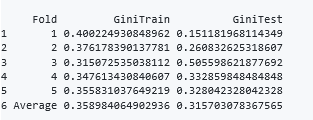
#Performing the 5 Fold cross validation
k.fold.cross.validation.glm(ms_train_data,"creditability",5,1)

Output:

#The KS test is performed on the distributions of the estimates for good and bad observations
Kolmogorov.Smirnov(ms_train_data,"creditability","PD")
Kolmogorov.Smirnov(ms_test_data,"creditability","PD")

The scorecards generally are revised in a long-term basis because the process creates an important operational cost. Therefore, the stability of the models reduces the need to revise. In addition, institutions want models that are stable since these models are used as input of many calculations like impairment, capital, risk weighted asset etc.

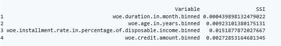
System Stability Index is a test used to measure the model and variable stability. SSI values above 0.25 indicate that variable stability is impaired.

#Variable stabilities are measured
SSI.calc.data(train_woe,test_woe,"creditability")

Output:

The HHI test measures the concentration of the master scale since the main purpose of the master scale is to differantiate the risk. Over 0.30 HHI values indicate high concentration. This may be due to modeling phase or the incorrect creation of the master scale.

#The HHI test is performed to measure the concentration of the master scale
Herfindahl.Hirschman.Index(master_scale,"Total.Observations")

Output:

0.1463665

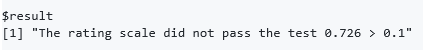
With the help of the “anchor.point” function, it is tested whether the default rate is compatible with average PD at the expected levels.

#Performing the Anchor point test
Anchor.point(master_scale,"PD","Total.Observations",0.30)

Output:

Chi square test can also be used as a calibration test. The “chisquare.test” function can be used to perform the test in the specified confidence level.

#The Chi-square test is applied on the master scale
chisquare.test(master_scale,"PD","Bad.Count","Total.Observations",0.90)

Output:

Binomial test can also be applied as a calibration test. The one-tail binomial test is usually used for IRB models, while the two-tail test is used for IFRS 9 models. But the two-tail test will be more convenient for general use, except for IRB.

#The Binomial test is applied on the master scale
master_scale$DR <- master_scale$Bad.Count/master_scale$Total.Observations
Binomial.test(master_scale,"Total.Observations","PD","DR",0.90,"one")

Output:

Modeling and model validation need to be managed to ensure continuity. When the R environment is managed correctly, this manageable modeling and validation environment can be provided easily by institutions.

Institutions are designing much more efficient business processes using open source environments such as R or Python with big data technologies. From this perspective, creditR offers organizational convenience to the application of modeling and validation methods.

End Notes

The creditR package provides users with a number of methods to perform traditional credit risk scoring, as well as some of those for testing model validity, which can also be applied to ML algorithms. Moreover, as the package provides automation in the application of the traditional methods, the operational costs for these processes can be reduced.

Furthermore, these models can be compared with the machine learning models in order to demonstrate that the ML models also meet the regulatory requirements, the meeting of which is the precondition for the application of ML models.

Bug Fixes and About the Author

Please inform the author about the errors you have encountered while using the package via the e-mail address that is shared below.

Ayhan Dis – Senior Risk Consultant

Ayhan Dis is a Senior Risk Consultant. He works on consulting projects like IFRS 9/IRB model development and validation,  as well as advanced analytics solutions including ML/DL in areas such as fraud analytics, customer analytics and risk analytics, using Python, R, Base SAS and SQL fluently.

Over the course of his work experience, he has worked with various types of data such as twitter, weather, credit risk, electric hourly price, stock price and customer data to offer solutions to his clients from sectors such as banking, energy, insurance, financing and  pharmaceutical industry.

As a data science enthusiast, he thinks that the real thrill of data science is not found in establishing one’s technical abilities; instead, it is found in blending data science together with big data to reveal insights which can be integrated with the bussiness processes, through artificial intelligence.

• https://github.com/ayhandis
•  https://www.linkedin.com/in/ayhandis/
•  [email protected]