This article was published as a part of the Data Science Blogathon.
This article happens to be a continuation of my last article on ‘Global Model Interpretability Techniques for Black Box Models’. Here we will discuss the feature importance technique – Accumulated Local Effects (ALE).
Introduction
With the availability of larger and richer data sets in many domains, black box supervised learning models like complex trees, random forests, boosted trees, nearest neighbors, support vector machines, etc. are gaining more importance as compared to the more transparent and more interpretable linear and logistic regression models to capture non-linear phenomena. Even if the purpose is purely predictive, understanding the effects of the predictors may still be quite important.
If the effect of a predictor violates intuition (e.g. if it appears from the supervised learning model that the risk of experiencing a cardiac event decreases as patients age), then this is either an indication that the fitted model is unreliable or that a surprising new phenomenon has been discovered. In addition, predictive models must be transparent in many regulatory environments, e.g. to demonstrate to regulators that consumer credit risk models do not penalize credit applicants based on age, race, etc.
When fitting black box supervised learning models, visualizing the main effects of the individual predictor variables and their low-order interaction effects is often important, and partial dependence (PD) plots are the most popular approach for accomplishing this.
However, they suffer from a stringent assumption: features have to be uncorrelated. In real-world scenarios, features are often correlated, whether because some are directly computed from others, or because observed phenomena produce correlated distributions. Hence, we need an unbiased technique, which ignores correlation among the features to a great extent. Accumulated Local Effects (ALE) can handle correlated predictors.
PDP vs M-plot vs Accumulated Local Effects (ALE)
In this article, we will explain a house price prediction example. For constructing a Partial Dependence Plot the following steps are to be followed:
- Select feature
- Define grid
- Per grid value:
- Replace feature with grid value
- Average predictions
- Draw the curve
For example, if we want to find the feature effects of sqft_living variable in comparison to the number of rooms, for the calculation of the first grid value of the PDP – say 40 m2 – we replace the sqft_living area for all instances by 40 m2, even for the houses with up to 8 rooms. The partial dependence plot includes these unrealistic houses in the feature effect estimation and pretends that everything is fine.
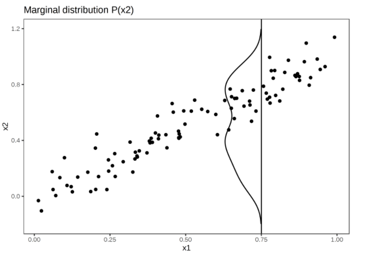
Strongly correlated features x1 and x2. To calculate the feature effect of x1 at 0.75, the PDP replaces x1 of all instances with 0.75, falsely assuming that the distribution of x2 at x1 = 0.75 is the same as the marginal distribution of x2 (vertical line). This results in unlikely combinations of x1 and x2 (e.g. x2=0.2 at x1=0.75), which the PDP uses for the calculation of the average effect.
To find the feature effects of correlated features, we can average over the conditional distribution of the feature, meaning at a grid value of x1, we average the predictions of instances with a similar x1 value. The solution for calculating feature effects using the conditional distribution is called Marginal Plots or M-Plots. But here also we have a problem. If we average the predictions of all houses of about 40 m2, we estimate the combined effect of the sqft_living and the number of rooms, due to the correlation. Even if the sqft_living has no effect on the price of a house, the M-plot will still show that an increase in the sqft_living increases the price of the house. The following plot shows for two correlated features how M-plots work.
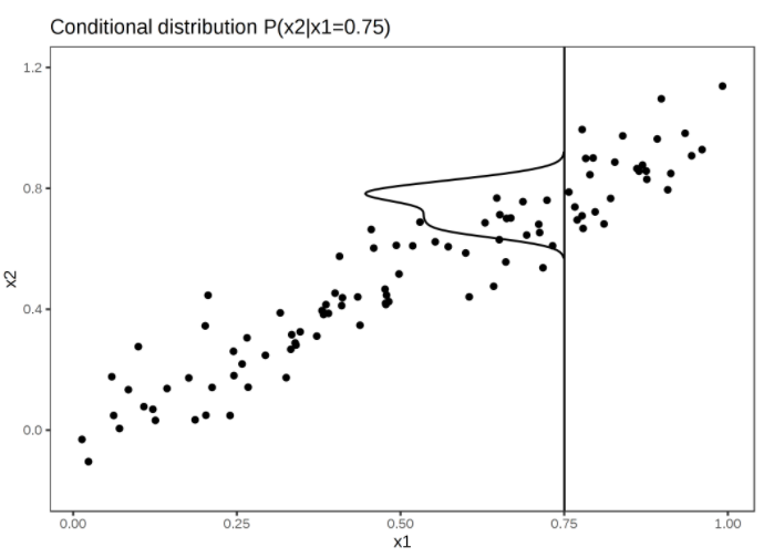
Strongly correlated features x1 and x2. M-Plots average over the conditional distribution. Here the conditional distribution of x2 at x1 = 0.75. Averaging the local predictions leads to mixing the effects of both features.
M-Plots avoid averaging predictions of unlikely data instances, but they mix the effect of a feature with the effects of all correlated features. ALE plots solve this problem by calculating the differences in predictions instead of averages. For the sqft_living variable at a value of 40 m2, the ALE technique uses all houses with about 40 m2, gets the model predictions pretending those houses were 41m2 minus the prediction pretending they were 39 m2. This gives us the pure feature effect of the sqft_living variable, without taking into account the effect of the correlated features. The following graphic provides intuition on how ALE plots are calculated:
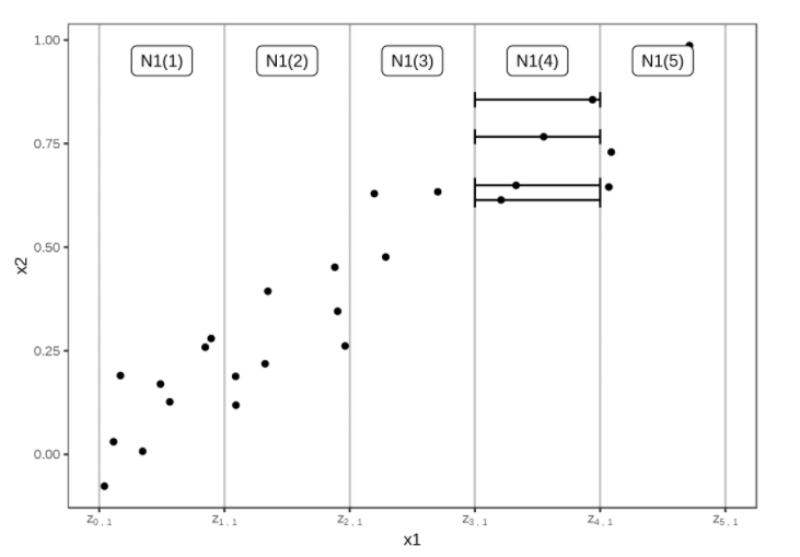
Calculation of ALE for feature x1, which is correlated with x2. First, we divide the feature into intervals (vertical lines). For the data instances (points) in an interval, we calculate the difference in the prediction when we replace the feature with the upper and lower limit of the interval (horizontal lines). These differences are later accumulated and centered, resulting in the ALE curve.
Implementation
Let us see how to implement ALE for a regression problem of predicting the house prices of King’s County. The dataset includes homes sold between May 2014 and May 2015. The Dataset has 21 features and 21613 observations. The dataset has been split into train, validation, and test, with the Test data having 2217 observations, as against train and validation data having 9761 and 9635 observations respectively. We train the model on the Train data. Evaluate several models on the Validation data. The final model is then used for predicting the target variable (Price) for the Test data.
We need to perform data cleaning and an exploratory data analysis to get to the model building stage. You can find the code here: Link to code
After cleaning the data and performing the EDA, we ended with the following variables:
- Predictors – bedrooms, bathrooms, log-transformed sqft_living, log-transformed sqft_lot, grade, log-transformed sqft_above, and yr_built.
- Target – Log transformed the prices of the houses.
We will perform a Multiple Linear Regression and a Random Forest model to understand the technique. We have used the ‘alibi‘ library.
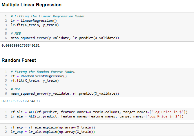
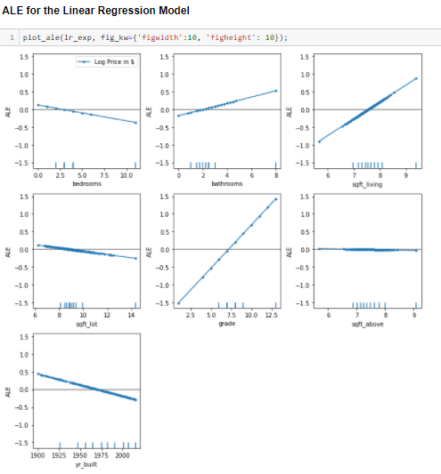
Next, we used the ALE technique for the Regression and the Random Forest model.
Interpretation
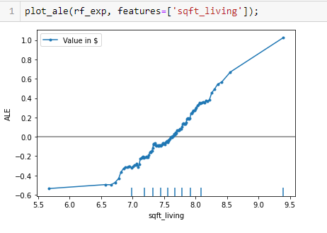
Let us consider the ALE plot of the sqft_living variable to interpret the results.
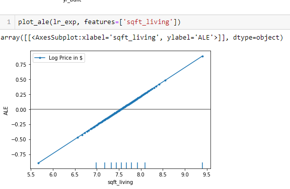
The ALE on the y_axis of the plot above is in the units of the prediction variable, i.e. the log-transformed price of the house in $. The ALE value for the point sqft-living = 8.5 is ~0.4, which has the interpretation that for neighborhoods for which the average log-transformed sqft_living is ~8.5 the model predicts an up-lift of log-transformed 0.4 units of price in $ due to the feature sqft_living with respect to the average prediction.
On the other hand, for the neighborhoods with an average log-transformed sqft_living lower than ~7.5, the feature effect on the prediction becomes negative, i.e. the log-transformed price in $ falls.
The ALE plots for the linear regression model are linear themselves—the feature effects are after all linear by definition. In fact, the slopes of the ALE lines are exactly the coefficients of the linear regression.
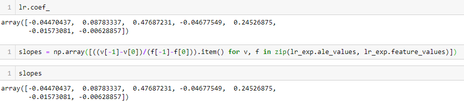
Thus the slopes of the ALE plots for linear regression have exactly the same interpretation as the coefficients of the learned model—global feature effects.
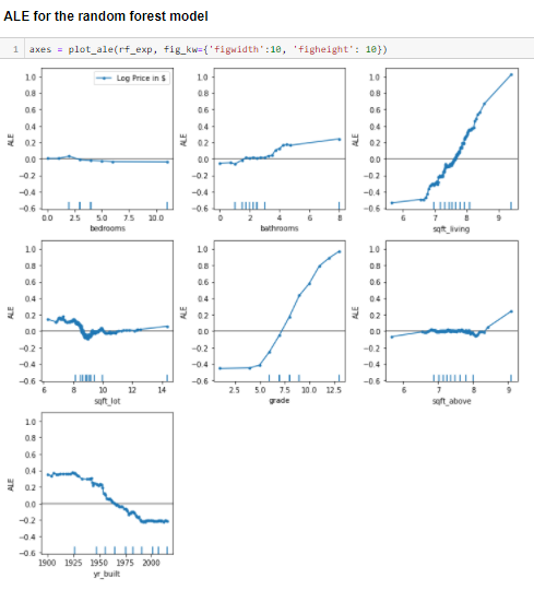
We can compare the ALE results for the two models.
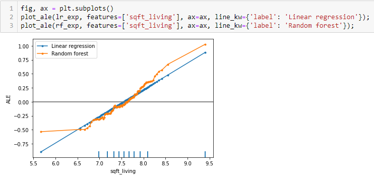
In the above plot, we can see Linear Regression feature effects of sqft_living are positively correlated, whereas Random Forest feature effects of sqft_living are not monotonic.
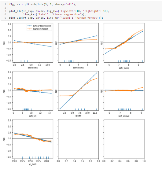
To compare multiple models and multiple features we can plot the ALE’s on a common axis that is big enough to accommodate all features of interest:
Advantages of Accumulated Local Effects(ALE) Plots
- ALE plots are unbiased, meaning they work with correlated features.
- ALE plots are computationally fast to compute.
- The interpretation of the ALE plot is clear.
Disadvantages of Accumulated Local Effects(ALE) Plots
- The implementation of ALE plots is complicated and difficult to understand.
- Interpretation still remains difficult if features are strongly correlated.
Conclusion
For visualizing the effects of the predictor variables in black box supervised learning models, PD plots are the most widely used method. The Accumulated Local Effects (ALE) plots are an alternative to the PD plots that work well on moderately correlated variables. This paper has been dedicated to ‘Sir Christoph Molnar‘. The motivation was his holistic work ‘A Guide for Making Black Box Models Explainable‘.
Reference
‘Visualizing the effects of predictor variables in black
box supervised learning models’ by Daniel W. Apley and Jingyu Zhu.


