Perform Regression Analysis with PyTorch Seamlessly!

Introduction

This is probably the 1000th article that is going to talk about implementing regression analysis using PyTorch. so how is it different?

Well, before I answer that let me write the series of events that led to this article. So, when I started learning regression in PyTorch, I was excited but I had so many whys and why nots that I got frustrated at one point. So, I thought why not start from scratch- understand the deep learning framework a little better and then delve deep into the complex concepts like CNN, RNN, LSTM, etc. and the easiest way to do so is taking a familiar dataset and explore as much as you can so that you understand the basic building blocks and the key working principle.

I have tried to explain the modules that are imported, why certain steps are mandatory, and how we evaluate a regression model in PyTorch.

So people, if you have just started or looking for answers as I did, then you are definitely in the right place. 🙂

Okay, so let’s start with the imports first.

Imports

import torch
import torch.nn as nn 

the torch.nn modules help us create and train neural networks. So definitely we need that. Let’s move on:

import pandas as pd
import numpy as np
import matplotlib.pyplot as plt
from sklearn.preprocessing import MinMaxScaler

They look familiar, right? We need them cause we have to do some preprocessing on the dataset we will be using.

Data

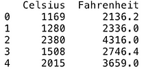
The dataset I am going to use is Celsius to Fahrenheit data which can be found here: link

Data preprocessing step 1: separate out the feature and the label

import pandas as pd
train_data = pd.read_csv('train_data.csv')
X_train = train_data.iloc[:,0].values
y_train = train_data.iloc[:,-1].values
print(X_train.shape)

Data preprocessing step 2: standardize the data as the values are very large and varied

So if you don’t do that for this particular case, then later while training the model, you will likely get inf or nan for loss values, meaning, the model cannot perform backpropagation properly and will result in a faulty model.

sc = MinMaxScaler()
sct = MinMaxScaler()
X_train=sc.fit_transform(X_train.reshape(-1,1))
y_train =sct.fit_transform(y_train.reshape(-1,1))

we have to make sure that X_train and y_train are 2-d.

Okay, so far so good. Now let’s enter into the world of tensors

Data preprocessing Step 3: Convert the numpy arrays to tensors

X_train = torch.from_numpy(X_train.astype(np.float32)).view(-1,1)
y_train = torch.from_numpy(y_train.astype(np.float32)).view(-1,1)

The view takes care of the 2d thing in tensor as reshape does in numpy.

Regression Model Building in PyTorch

input_size = 1
output_size = 1

input= celsius

output = fahrenheit

Define layer

class LinearRegressionModel(torch.nn.Module):

    def __init__(self):
        super(LinearRegressionModel, self).__init__()
        self.linear = torch.nn.Linear(1, 1)  # One in and one out

    def forward(self, x):
        y_pred = self.linear(x)
        return y_pred

Or we could have simply done this(since it is just a single layer)

model = nn.Linear(input_size , output_size)

In both cases, we are using nn.Linear to create our first linear layer, this basically does a linear transformation on the data, say for a straight line it will be as simple as y = w*x, where y is the label and x, the feature. Of course, w is the weight. In our data, celsius and fahrenheit follow a linear relation, so we are happy with one layer but in some cases where the relationship is non-linear, we add additional steps to take care of the non-linearity, say for example add a sigmoid function.

Define loss and optimizer

learning_rate = 0.0001
l = nn.MSELoss()
optimizer = torch.optim.SGD(model.parameters(), lr =learning_rate )

as you can see, the loss function, in this case, is “mse” or “mean squared error”. Our goal will be to reduce the loss and that can be done using an optimizer, in this case, stochastic gradient descent. That SGD needs initial model parameters or weights and a learning rate.

Okay, now let’s start the training.

Training

num_epochs = 100for epoch in range(num_epochs):
    #forward feed
    y_pred = model(X_train.requires_grad_())

    #calculate the loss
    loss= l(y_pred, y_train)

    #backward propagation: calculate gradients
    loss.backward()

    #update the weights
    optimizer.step()

    #clear out the gradients from the last step loss.backward()
    optimizer.zero_grad()
    
    print('epoch {}, loss {}'.format(epoch, loss.item()))

forward feed: in this phase, we are just calculating the y_pred by using some initial weights and the feature values.

loss phase: after the y_pred, we need to measure how much prediction error happened. We are using mse to measure that.

backpropagation: in this phase gradients are calculated.

step: the weights are now updated.

zero_grad: finally, clear the gradients from the last step and make room for the new ones.

Evaluation

predicted = model(X_train).detach().numpy()

detach() is saying that we do not need to store gradients anymore so detach that from the tensor. Now, let’s visualize the model quality with the first 100 data points.

plt.scatter(X_train.detach().numpy()[:100] , y_train.detach().numpy()[:100])
plt.plot(X_train.detach().numpy()[:100] , predicted[:100] , "red")
plt.xlabel("Celcius")
plt.ylabel("Farenhite")
plt.show()

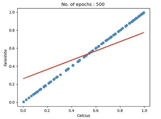
Notice, how with the increase in the number of the epochs, the predictions are getting better. There are multiple other strategies to optimize the network, for example changing the learning rate, weight initialization techniques, and so on.

Lastly, try with a known celsius value and see if the model is able to predict the fahrenheit value correctly. The values are transformed, so make sure you do a sc.inverse_transform() and sct.inverse_transform() to get the actual values.

Thank you for reading this article. Please do leave a comment or share your feedback. 🙂

References:

About the Author

I am Dipanwita Mallick, currently working as a Senior Data Scientist at Hewlett Packard Enterprise.  My work involves building and productionizing predictive models in the HPC & AI domain to efficiently and effectively use HPC clusters, supercomputers expanded over 10,000 cores with high bandwidth, low latency interconnects, several petabytes of data storage and databases.

Prior to that I have worked with Cray Inc. in Seattle and United Educators in Washington DC as a Data Scientist.

I have also done my Master’s in Data Science from Indiana University, Bloomington.