Employee Attrition Analysis using Logistic Regression with R

This article was published as a part of the Data Science Blogathon.

“To win in the market place you must win in the workplace” –Steve Jobs, founder of Apple Inc.

Introduction

Nowadays, employee attrition became a serious issue regarding a company’s competitive advantage. It’s very expensive to find, hire and train new talents. It’s more cost-effective to keep the employees a company already has. A company needs to maintain a pleasant working atmosphere to make their employees stay in that company for a longer period. A few years back it was done manually but it is an era of machine learning and data analytics. Now, a company’s HR department uses some data analytics tool to identify which areas to be modified to make most of its employees to stay.

Why are we using logistic regression to analyze employee attrition?

Whether an employee is going to stay or leave a company, his or her answer is just binomial i.e. it can be “YES” or “NO”. So, we can see our dependent variable Employee Attrition is just a categorical variable. In the case of a dependent categorical variable, we can not use linear regression, in that case, we have to use “LOGISTIC REGRESSION“.

Methodology

Here, I am going to use 5 simple steps to analyze Employee Attrition using R software

1. DATA COLLECTION
2. DATA PRE PROCESSING
3. DIVIDING THE DATA into TWO PARTS “TRAINING” AND “TESTING”
4. BUILD UP THE MODEL USING “TRAINING DATA SET”
5. DO THE ACCURACY TEST USING “TESTING DATA SET”

Data Exploration

This data set is collected from the IBM Human Resource department. The dataset contains 1470 observations and 35 variables. Within 35 variables “Attrition” is the dependent variable.

A quick look at the dataset:

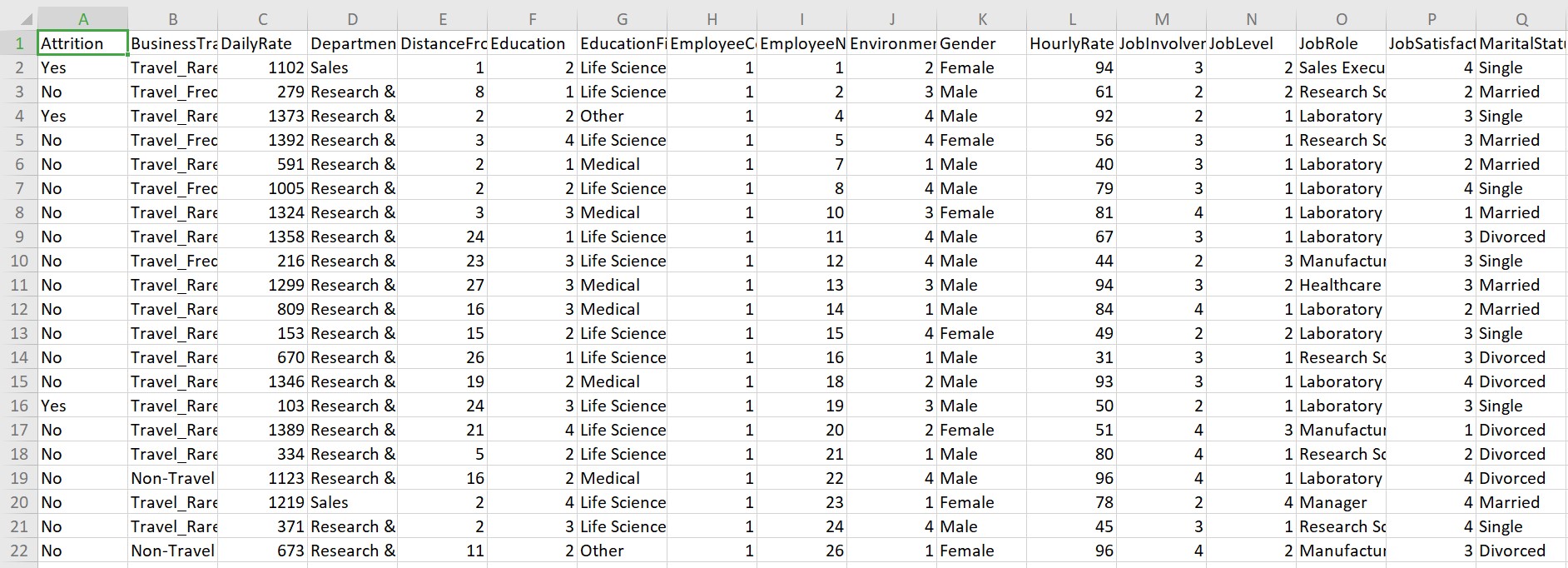
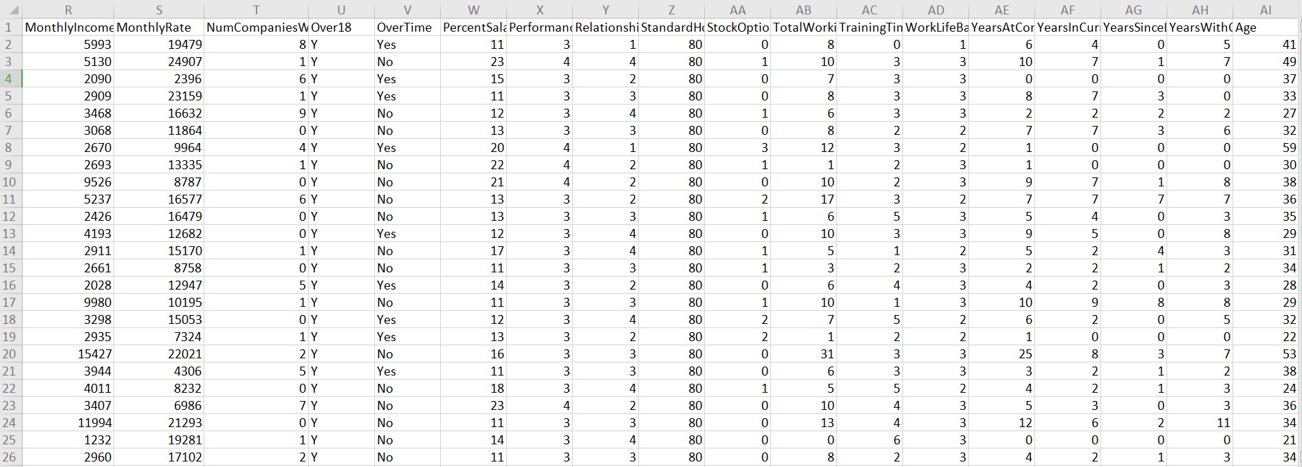
Take a look:

Data preparation

• Detect the missing values:

  We have to see if there are any missing values in the dataset.

  anyNA(JOB_Attrition)

  Result: FALSE; i.e. there are no missing values in our data set ” JOB_Attrition”

• Change the data types:

  First of all, we have to change the data type of the dependent variable “Attrition”. It is given as “Yes” and “No” form i.e. it is a categorical variable. To make a proper model we have to convert it into numeric form. To do so, we will assign value 1 to “Yes” and value 0 to “No” and convert it into numeric.

  JOB_Attrition$Attrition[JOB_Attrition$Attrition=="Yes"]=1
  JOB_Attrition$Attrition[JOB_Attrition$Attrition=="No"]=0
  JOB_Attrition$Attrition=as.numeric(JOB_Attrition$Attrition)

  Next, we will change all “character” variables into “Factor”

  There are 8 character variables: Business Travel, Department, Education, Education Field, Gender, Job role, Marital Status, Over Time. There column numbers are 2,4,6,7,11,15,17,22 respectively.

  JOB_Attrition[,c(2,4,6,7,11,15,17,22)]=lapply(JOB_Attrition[,c(2,4,6,7,11,15,17,22)],as.factor)

  Lastly, there is one other variable ” Over 18″ which has all inputs as “Y”. It is also a character variable. We will transform into numeric as it has only one level so transforming into factor will not provide a good result. To do so, we will assign value 1 to “Y” and transform it into numeric.

  JOB_Attrition$Over18[JOB_Attrition$Over18=="Y"]=1
  JOB_Attrition$Over18=as.numeric(JOB_Attrition$Over18)

Splitting the dataset into “training” and “testing”

In any regression analysis, we have to split the dataset into 2 parts:

1. TRAINING DATA SET
2. TESTING DATA SET

With the help of the Training data set we will build up our model and test its accuracy using the Testing Data set.

set.seed(1000)
ranuni=sample(x=c("Training","Testing"),size=nrow(JOB_Attrition),replace=T,prob=c(0.7,0.3))
TrainingData=JOB_Attrition[ranuni=="Training",]
TestingData=JOB_Attrition[ranuni=="Testing",]
nrow(TrainingData)
nrow(TestingData)

We have successfully split the whole data set into two parts. Now we have 1025 Training data & 445 Testing data.

Building up the model

We are now going to build up the model following some simple steps as follows:

1. Identify the independent variables
2. Incorporate the dependent variable “Attrition” in the model
3. Transform the data type of model from “character” to “formula”
4. Incorporate TRAINING data into the formula and build the model

independentvariables=colnames(JOB_Attrition[,2:35])
independentvariables
Model=paste(independentvariables,collapse="+")
Model
Model_1=paste("Attrition~",Model)
Model_1
class(Model_1)
formula=as.formula(Model_1)
formula

Output:

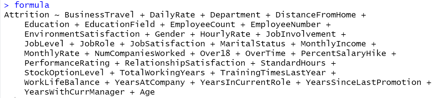
Next, we will incorporate “Training Data” into the formula using the “glm” function and build up a logistic regression model.

Trainingmodel1=glm(formula=formula,data=TrainingData,family="binomial")

Now, we are going to design the model by the “Stepwise selection” method to fetch significant variables of the model. Execution of the code will give us a list of output where the variables are added and removed based on our significance of the model. The AIC value at each level reflects the goodness of the respective model. As the value keeps dropping it leads to a better fitting logistic regression model.

The application of the summary on the final model will give us the list of final significant variables and their respective important information.

Trainingmodel1=step(object = Trainingmodel1,direction = "both")
summary(Trainingmodel1)

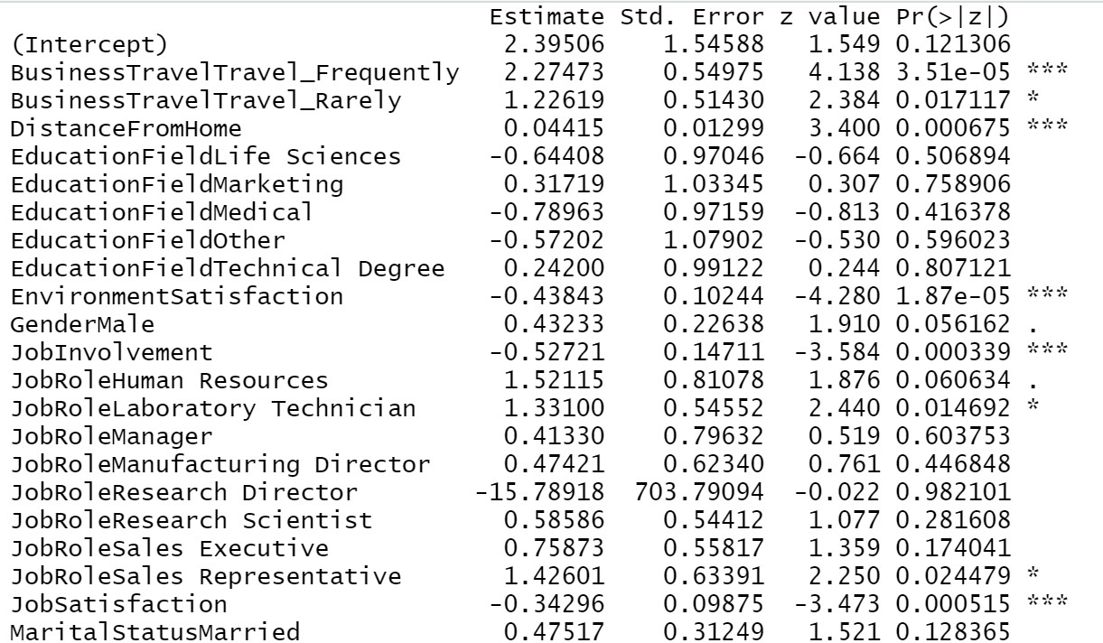
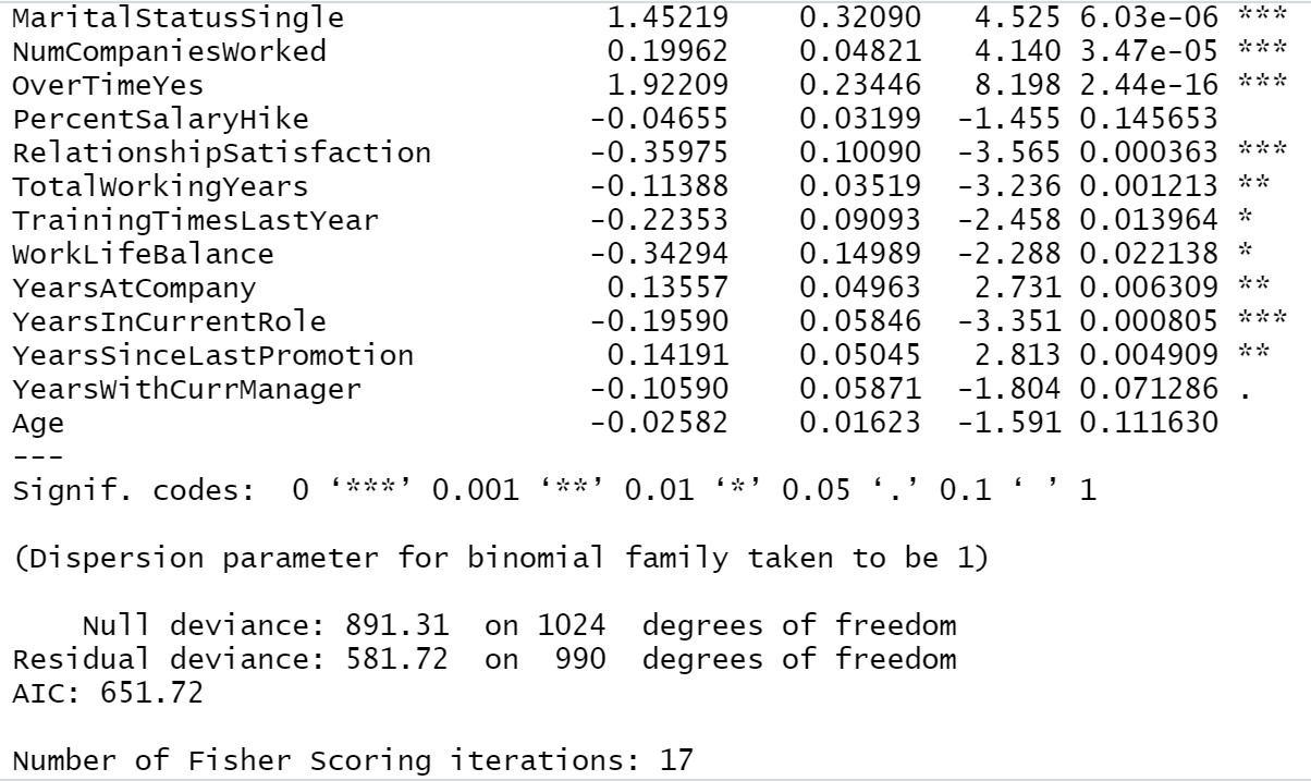
From our above result we can see, Business travel, Distance from home, Environment satisfaction, Job involvement, Job satisfaction, Marital status, Number of companies worked, Over time, Relationship satisfaction, Total working years, Years at the company, years since last promotion, years in the current role all these are most significant variables in determining employee attrition. If the company mostly looks after these areas then there will be a lesser chance of losing an employee.

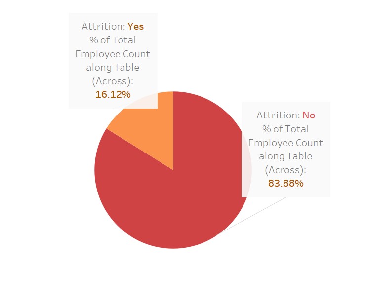
A quick visualization to see how much these variables affect “attrition”

 

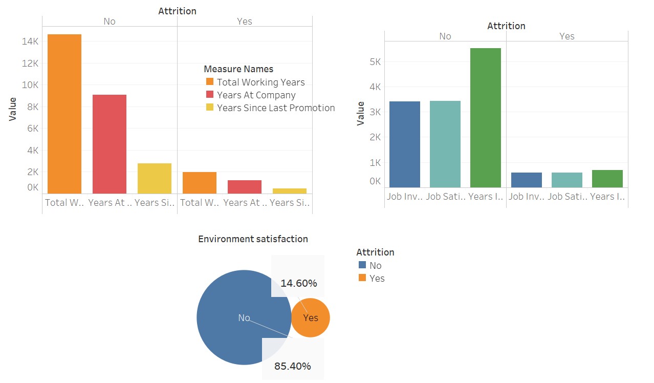
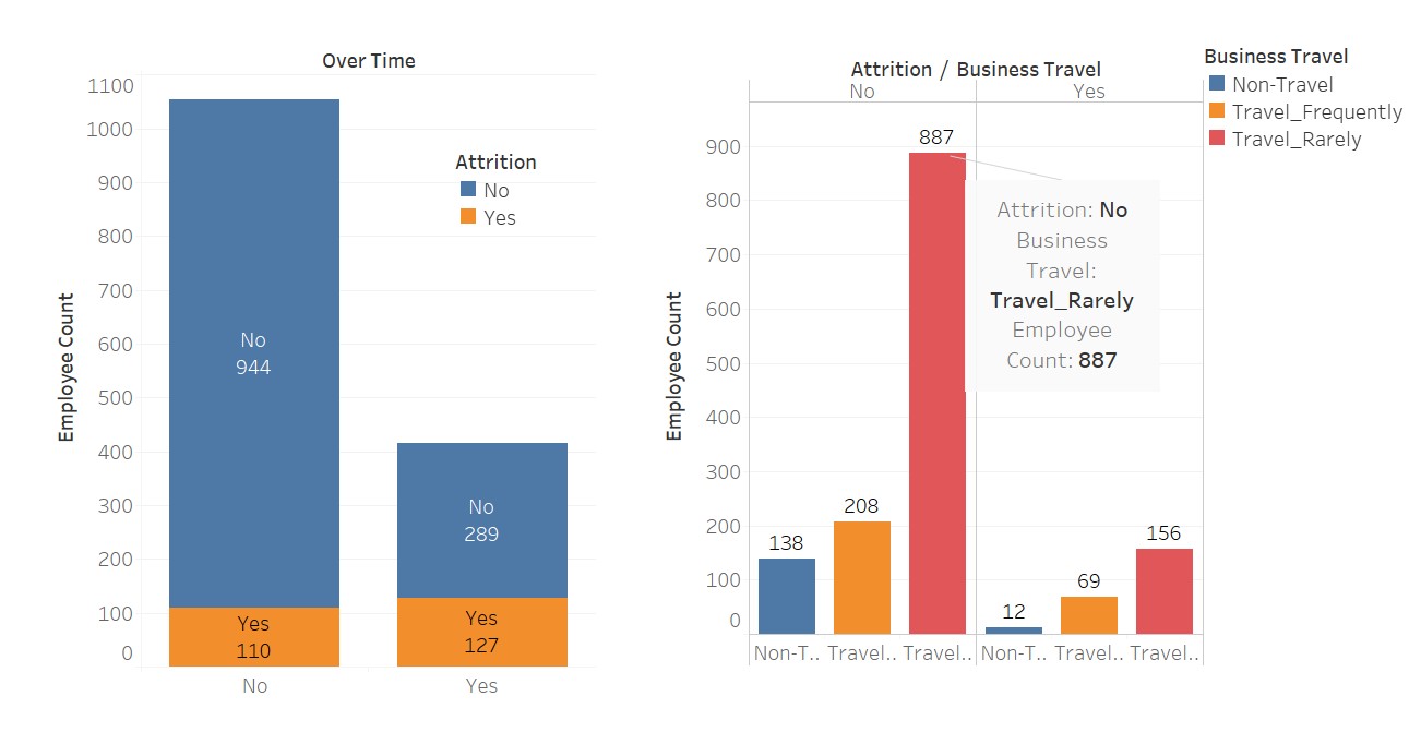
Here I have used Tableau for these visualizations; isn’t it beautiful? This software just makes our work easier.

Now, we can perform the Hoshmer-Lemeshow goodness of fit test on the data set, to judge the accuracy of the predicted probability of the model.

The hypothesis is:

H0: The model is a good fit.

H1: The model is not a good fit.

If, p-value>0.05 we will accept H0 and reject H1.

To perform the test in R we need to install the mkMisc package.

HLgof.test(fit=Trainingmodel1$fitted.values,obs=Trainingmodel1$y)

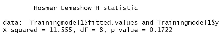
Here, we can see the p-value is greater than 0.05, hence we will accept H0. Now, it is proved that our model is a well fitted one.

Generating a ROC curve for training data

Another technique to analyze the goodness of fit of logistic regression is the ROC measures(Receiver Operating characteristics). The ROC measures are sensitivity, 1-Specificity, False Positive, and False Negative. The two measures we use extensively are Sensitivity and Specificity. The sensitivity measures the goodness of accuracy of the model while specificity measures the weakness of the model.

To do this in R we need to install a package pROC.

troc=roc(response=Trainingmodel1$y,predictor = Trainingmodel1$fitted.values,plot=T)
troc$auc

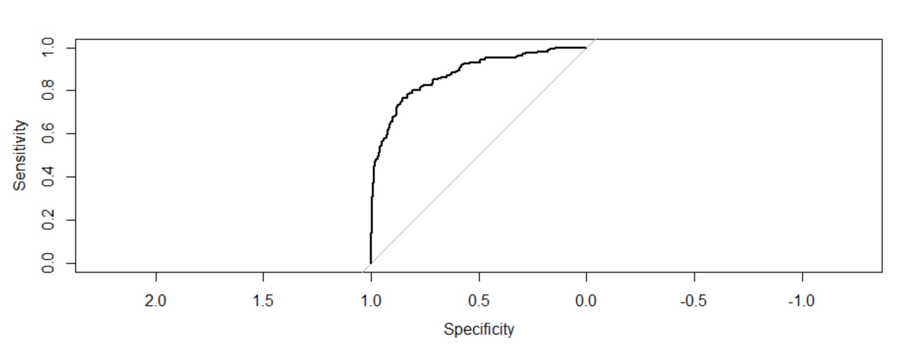
The area under the curve: 0.8759

Interpretation of the figure:

The plot of these two measures gives us a concave plot which shows as sensitivity is increasing 1-specificity is increasing but at a diminishing rate. The C-value(AUC) or the value of the concordance index gives the measure of the area under the ROC curve. If c=0.5 then it would have meant that the model can not perfectly discriminate between 0 and 1 responses. Then it implies that the initial model can not perfectly say which employees are going to leave and who are going to stay.

But, here we can see our c-value is far greater than 0.5. It is 0.8759. Our model can perfectly discriminate between 0 and 1. Hence, we can successfully conclude it is a well-fitted model.

Creating the classification table for the training data set:

trpred=ifelse(test=Trainingmodel1$fitted.values>0.5,yes = 1,no=0)
table(Trainingmodel1$y,trpred)

The above code states, the predicted value of the probability greater than 0,.5 then the value of the status is 1 else it is 0. based on this criterion this code relabels ‘Yes’ and ‘No’ Responses of “Attrition”. Now, it is important to understand the percentage of predictions that match the initial belief obtained from the data set. Here we will compare (1-1) and (0-0) pair.

We have 1025 training data. We have predicted {(839+78)/1025}*100=89% correctly.

Comparing the result with testing data:

We will now compare the model with testing data. It is much like an accuracy test.

testpred=predict.glm(object=Trainingmodel1,newdata=TestingData,type = "response")
testpred
tsroc=roc(response=TestingData$Attrition,predictor = testpred,plot=T)
tsroc$auc

Now, We have incorporated Testing data into the training model and will see the ROC.

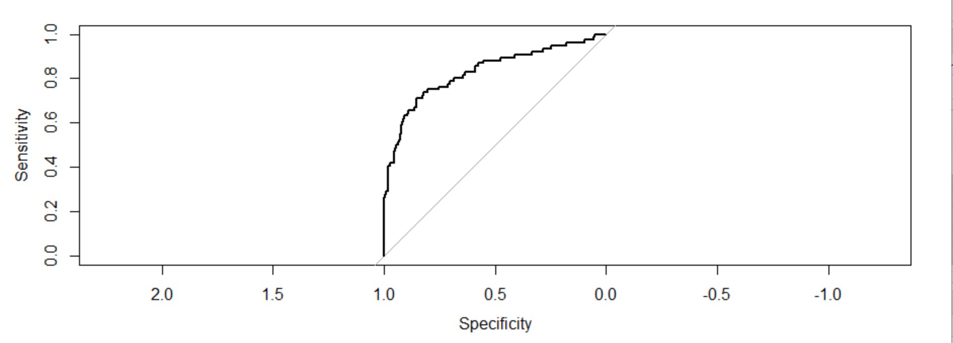
The area under the curve: 0.8286(c-value). It is also far higher than 0.5. It is also a well-fitted model.

Creating the classification table for the testing data set

testpred=ifelse(test=testpred>0.5,yes=1,no=0)
table(TestingData$Attrition,testpred)

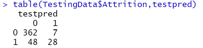
We have 445 Testing data. we have correctly predicted {(362+28)/445}*100=87.64%.

Consequently, we can say, our logistic regression model is a very good fitted model. Any employee attrition data set can be analyzed using this model.

What do you think is it a good model? Comment below

CONCLUSION:

We have successfully learned how to analyze employee attrition using “LOGISTIC REGRESSION” with the help of R software. Only with a couple of codes and a proper data set, a company can easily understand which areas needed to look after to make the workplace more comfortable for their employees and restore their human resource power for a longer period.

featured image is taken from trainingjournal.com

Link to my LinkedIn profile:

https://www.linkedin.com/in/tiasa-patra-37287b1b4/

TIASA