Dynamic Bus Fare Pricing Comparison and Detection

This article was published as a part of the Data Science Blogathon.

Introduction

Online bus ticketing in India has taken the bus service industry by storm with multiple players catering to different customer segments, geographies and proving value-added services such as insurance, various amenities, etc. Once a technologically backward and resource-intensive public transport industry is now transformed into a travel industry behemoth within a decade. The major players in the industry are Redbus, Makemytrip, Goibibo, EaseMyTrip all fighting to capture market share and assert dominance.

Though plenty of levers is available to capture market share, pricing still remains the most important in India. Pricing can make or break bus operators. In an industry that already has high operating costs and low margins, getting the price right is the most fundamental decision that every operator has to take, either a large or a smaller one. One Bain study found that 78% of B2C firms believe they can still improve their pricing strategies.

Ideally, a sleeper bus has 34 seats, lets’s consider a bus operator that has 3 buses and plans topline growth. Two major options prevail, either raise the number of seats or raise prices. A 10% increase in price leads to a 2% increase in topline compared to a 10% increase in volume leads to a 1% increase. This example might not cover all the bases but provides sufficient evidence to support the power of pricing.

What pricing strategies can be used?

1. Zonal Pricing – Simple and direct pricing based on zones. Used by government public transport.
2. Distance Pricing – Pricing based on distance travelled, used majorly by buses on hire, tourist operators.
3. Origin destination Pricing – Based on the destination, if a major tourist destination, then higher prices.
4. Seasonal Pricing – Based on the season.
5. Last-minute Pricing – Some operators drastically reduce or increase prices to increase volumes.
6. Dynamic Pricing – Most common in eCommerce where marketplaces have higher price setting flexibility, sparse adoption in the bus service industry.

This article explores the world of online bus tickets pricing. We will cover the following:

1. Problem statement
2. Explore dataset
3. Data preprocessing
4. Exploratory data analysis
5. Exploring feasible solutions
6. Test for accuracy and evaluation

1. Problem Statement:

Large bus operators have higher pricing power as they are already well placed in the market. The problem statement is to identify operators who are pricing independently(ideally large operators) and operators who are followers. Identifying market leaders through a data-based approach helps businesses serve these players better. As resources are scarce, the question is on which operator should the company utilize its resources better? Other use cases of this analysis can be used for internal strategic decision making and can have a positive impact on the long term relationships between operators and online ticketing platforms.

Problem Statement – Identify price-setters and followers. 

2. Explore Dataset:

Data can be downloaded from here.

bus_fare_df = pd.read_csv("https://raw.githubusercontent.com/chrisdmell/DataScience/master/data_dump/07_bus_fare_pricing/PricingData.csv") 
display(bus_fare_df.head())
display(bus_fare_df.shape)
display(bus_fare_df.describe())
display(bus_fare_df.dtypes)

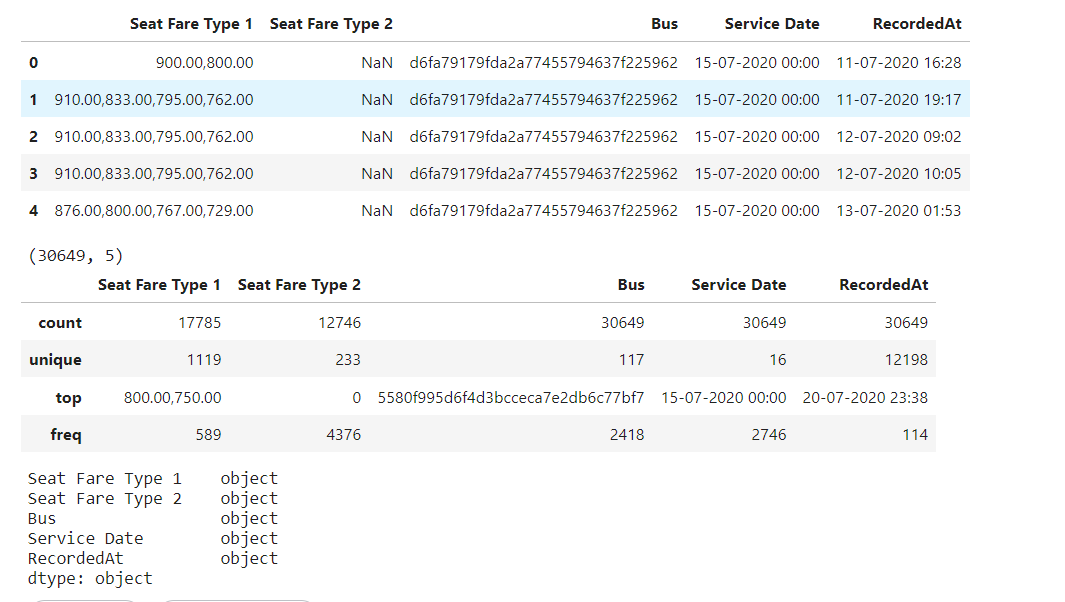
• Seat Fare Type 1 – Type 1 seat fare.
  • Seat type 1 has a different set of prices.
  • Need to clean it and identify a single price, such that this analysis can be easy and less complicated.
• Seat Fare Type 2 – Type 2 seat fare.
  • Similar to Seat Fare Type 1.
• Bus – Bus unique identifier.
• Service Date – Journey date.
  • Convert to pandas timestamp and get day of the week, month, year etc information.
• RecordedAt – Pricing recorded date, price captures by the system.
  • Similar to service date.

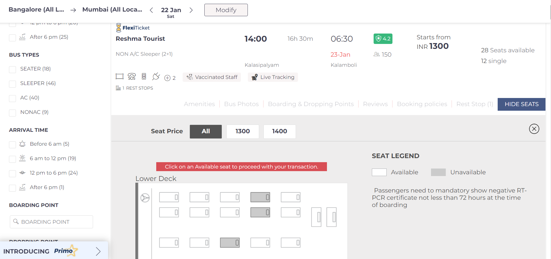
Modern ticketing platforms enrich customer experience through robust UI. On the left-hand side, there are the filters such as bus types, amenities, the top has information about the bus timings, prices and the bottom space provides seat selected capability.

3. Data Preprocessing: 

Functions to clean pricing columns –

def clean_seat(x):
    '''
    input is a string object and not a list
    '''
#     a = [float(sing_price)  for  price in x for sing_price in price.split(",")]
#     a = [sing_price  for  price in x for sing_price in price.split(",")]
#     return sum(a)/len(a)
    a = [float(price) for price in x.split(",")]
    return sum(a)/len(a)
def average_s1_s2_price(s1, s2):
    '''
    pandas series as input 
    for price 1 and price 2 all 4 combination covered. 
    '''
    price_output = []
#     for i in range(len(s1)):
    if (s1 == 0) & (s2 == 0):
        return 0
    elif (s1 == 0) & (s2 !=0 ):
        return s2
    elif (s1 != 1) & (s2 ==0 ):
        return s1
    else :
        return (s1+s2)/2
#     return price_output

• Calculate the average fare per bus, having one data point is easier than multiple.
• Backfill prices so that missing values can be replaced.
• Convert seat fare type 1 and seat fare type 2 to string and replace null

bus_fare_df = bus_fare_df.sort_values(by = ["Bus","Service_Date","RecordedAt" ])
# display(bus_fare_df.head())
test = bus_fare_df[["Bus","Service_Date","RecordedAt","Seat_Fare_Type_1_average" ]].sort_values(by = ["Bus","Service_Date","RecordedAt" ])
test = test[["Bus","Service_Date","Seat_Fare_Type_1_average" ]]
test["Seat_Fare_Type_1_average_impute"] = test.groupby(["Bus","Service_Date" ]).transform(lambda x: x.replace(to_replace=0, method='ffill'))
display(test.shape)
display(bus_fare_df.shape)
test2 = bus_fare_df[["Bus","Service_Date","RecordedAt","Seat_Fare_Type_2_average" ]].sort_values(by = ["Bus","Service_Date","RecordedAt" ])
test2 = test2[["Bus","Service_Date","Seat_Fare_Type_2_average" ]]
test2["Seat_Fare_Type_2_average_impute"] = test2.groupby(["Bus","Service_Date" ]).transform(lambda x: x.replace(to_replace=0, method='ffill'))
display(test2.shape)
# display(bus_fare_df.shape)
bus_fare_df["Seat_Fare_Type_1_average_impute_ffil"] = test["Seat_Fare_Type_1_average_impute"] 
bus_fare_df["Seat_Fare_Type_2_average_impute_ffil"] = test2["Seat_Fare_Type_2_average_impute"] 
# display(bus_fare_df.head())
#############################################################################################################################
test = bus_fare_df[["Bus","Service_Date","RecordedAt","Seat_Fare_Type_1_average" ]].sort_values(by = ["Bus","Service_Date","RecordedAt" ])
test = test[["Bus","Service_Date","Seat_Fare_Type_1_average" ]]
test["Seat_Fare_Type_1_average_impute_bfil"] = test.groupby(["Bus","Service_Date" ]).transform(lambda x: x.replace(to_replace=0, method='bfill'))
display(test.shape)
test2 = bus_fare_df[["Bus","Service_Date","RecordedAt","Seat_Fare_Type_2_average" ]].sort_values(by = ["Bus","Service_Date","RecordedAt" ])
test2 = test2[["Bus","Service_Date","Seat_Fare_Type_2_average" ]]
test2["Seat_Fare_Type_2_average_impute_bfil"] = test2.groupby(["Bus","Service_Date" ]).transform(lambda x: x.replace(to_replace=0, method='bfill'))
display(test2.shape)
bus_fare_df["Seat_Fare_Type_1_average_impute_bfill"] = test["Seat_Fare_Type_1_average_impute_bfil"] 
bus_fare_df["Seat_Fare_Type_2_average_impute_bfill"] = test2["Seat_Fare_Type_2_average_impute_bfil"] 
# display(bus_fare_df.hea
#############################################################################################################################
test_a = bus_fare_df[["Bus","Service_Date","RecordedAt","average_price_s1_s2" ]].sort_values(by = ["Bus","Service_Date","RecordedAt" ])
test_a = test_a[["Bus","Service_Date","average_price_s1_s2" ]]
test_a["average_price_s1_s2_bfil"] = test_a.groupby(["Bus","Service_Date" ]).transform(lambda x: x.replace(to_replace=0, method='bfill'))
display(test_a.shape)
test_f = bus_fare_df[["Bus","Service_Date","RecordedAt","average_price_s1_s2" ]].sort_values(by = ["Bus","Service_Date","RecordedAt" ])
test_f = test_f[["Bus","Service_Date","average_price_s1_s2" ]]
test_f["average_price_s1_s2_ffil"] = test_f.groupby(["Bus","Service_Date" ]).transform(lambda x: x.replace(to_replace=0, method='ffill'))
display(test_f.shape)
bus_fare_df["average_price_s1_s2_bfill"] = test_a["average_price_s1_s2_bfil"] 
bus_fare_df["average_price_s1_s2_ffill"] = test_f["average_price_s1_s2_ffil"] 
# display(bus_fare_df.head())
#############################################################################################################################
bus_fare_df['average_price_s1_s2_filled'] = bus_fare_df.apply(lambda x: average_s1_s2_price(x.average_price_s1_s2_ffill, x.average_price_s1_s2_bfill), axis=1)

• Create flags for buses with only Rs 0 as price point, these could be cancelled buses.
• average_price_s1_s2_filled is the final average price point.
• The level of data/detail(LOD) is Bus x Service_Date x RecordedAt
• The preprocessing step creates all the cleaned columns and features.
• The code can be downloaded from here as well.

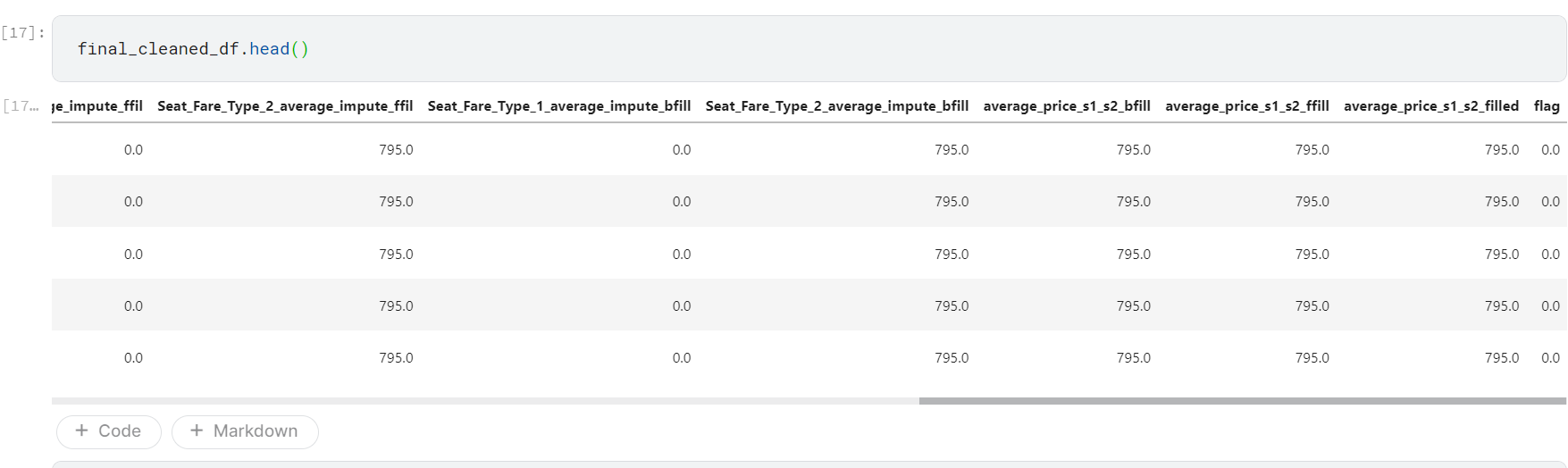
Screenshot: Author

4. Exploratory Data Analysis

EDA is all about asking as many relevant questions as possible and getting answers through data. EDA on its own might not help solve the business problem but will provide valuable explanations as to why something things are the way they are. It also helps identify important features in a dataset and filter out discrepancies.

As only pricing data is available, certain assumptions help narrow down the analysis. :

1. All operators are charged a similar commission.
2. All operators have similar ratings/amenities.
3. All operators run on the same routes, covering similar distances.
4. All operators have similar boarding and destination points.
5. All operators have a similar couponing/discounting policy.

Null hypothesis – All operators price independently and there are no price-setters or followers.

Alternate hypothesis – Not all operators price independently and there are price setters and followers.

EDA problem statements and probable business intelligence gained by answering them :

1. Percentage change between the initial price and final price?
   1. Do operators increase or decrease price over time – this information can be leveraged to help bus operators identify opportunities to keep prices constant instead of reducing.
   2. It also provides initial impetus and validates our problem statement.
2. Days between price listing and journey date:
   1. Identify the perfect window for listing. Is 10 days before the journey date too short or is it 30 days too long? Does the early bird always get the worm? The optimized window saves cost, If all seats are not filled within the time then it’s a loss, if all seats are filled before time, then an opportunity is lost, which turns out to be an opportunity cost.
3. Daily average prices across platform vs bus operators:
   1. Identify market price expectations, and improve pricing decisions.
4. Price bucketing of buses:
   1. Descriptive statistics.
   2. Identify competition and deploy tactics to mitigate losses due to competitive pricing.
5. Day of the week analysis on price:
   1. Weekend weekday analysis, to improve pricing decisions.
6. Price elasticity across the platform:
7. Based on prices, identify the different seats available:
   1. Try to gauge price sensitivity on the type of seating.

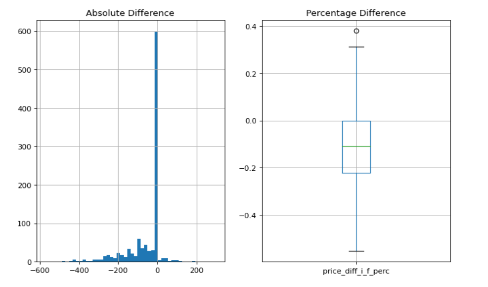
Percentage change between the initial price and final price?

• For 60% of Bus X Service_Date combinations change in the initial and final price is 0.
• The remaining 40% buses majorly have seen a decrease in final prices.
• The box and whisker plot shows on average 10% decrease in final price.
• Operators list higher prices eventually to reduce them over time.
• MOM(month on month) boxplot of the same would shed some light on how seasonality can affect price change.

Code:

one_df_002 = pd.merge(one_df,final_cleaned_df[["Bus","Service_Date","RecordedAt", "average_price_s1_s2_filled"]], how = "left" , left_on = ["Bus","Service_Date","min"], right_on =["Bus","Service_Date","RecordedAt"], 
                     suffixes=('_left', '_right'))
one_df_003 = pd.merge(one_df_002,final_cleaned_df[["Bus","Service_Date","RecordedAt", "average_price_s1_s2_filled"]], how = "left" , left_on = ["Bus","Service_Date","max"], right_on =["Bus","Service_Date","RecordedAt"], 
                     suffixes=('_left', '_right'))
one_df_003["price_diff_i_f"] = one_df_003.average_price_s1_s2_filled_right - one_df_003.average_price_s1_s2_filled_left
one_df_003["price_diff_i_f_perc"] = one_df_003.price_diff_i_f / one_df_003.average_price_s1_s2_filled_left
one_df_004 = one_df_003[["Bus","Service_Date", "price_diff_i_f"]].drop_duplicates()
one_df_005 = one_df_003[["Bus","Service_Date", "price_diff_i_f_perc"]].drop_duplicates()
one_df_005.boxplot(column = ["price_diff_i_f_perc"])
one_df_004.price_diff_i_f.hist(bins = 50)

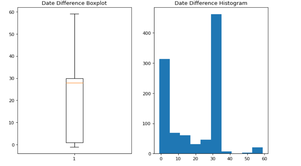
Days between price listing and journey date

• On average operators list 30 days in advance on the platform.
• 75% list on or before 30 days.
• Final 25% percentile list between 30 and 60 days.
• It would be interesting to see if buses listed for longer periods operate at higher volumes as compared to average.

Code:

groups = final_cleaned_df.groupby(["Bus","Service_Date_new"]).RecordedAt_new                           
min_val = groups.transform(min)
one_df = final_cleaned_df[(final_cleaned_df.RecordedAt_new==min_val) ]
one_df["date_diff"] = one_df.Service_Date_new - one_df.RecordedAt_new
figure(figsize=(10, 6), dpi=80)
plt.subplot(1, 2, 1)
plt.title("Date Difference Boxplot")
plt.boxplot(one_df.date_diff.astype('timedelta64[D]'))
plt.subplot(1, 2, 2)
plt.title("Date Difference Histogram")
plt.hist(one_df.date_diff.astype('timedelta64[D]'))

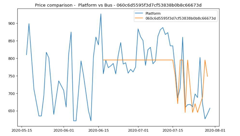
Daily average prices across platform vs bus operators

• The flat orange price line till 20200715 is backfilled, hence appears to be constant.
• This provides a view of the platform average prices vs a single bus operator.
• Near the journey period, there is a shift of the peak to the right.

Code:

plot_1 = bus_fare_df[bus_fare_df["average_price_s1_s2_filled"] !=0].groupby(["RecordedAt_date_only"]).agg({"average_price_s1_s2_filled":np.mean})
figure(figsize=(10, 6), dpi=80)
plt.plot(plot_1.index, plot_1.average_price_s1_s2_filled,label = "Platform")
plot_2 = bus_fare_df[(bus_fare_df["average_price_s1_s2_filled"] !=0)&(bus_fare_df["Bus"] =="060c6d5595f3d7cf53838b0b8c66673d")].groupby(["RecordedAt_date_only"]).agg({"average_price_s1_s2_filled":np.mean})
plt.plot(plot_2.index, plot_2.average_price_s1_s2_filled, label = "060c6d5595f3d7cf53838b0b8c66673d")
plt.show()

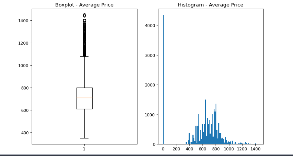
Price bucketing of buses

• Using price buckets, the different types of seats available can be identified.
• For operators, helps understand competition, and provide more information on how to position themselves in the market.
• Understanding the market helps set internal pricing business rules and guardrails.
• The lowest price is 350, the highest is 1449.
• The average is 711 and the 50 percentile is 710. Proof that the Central Limit Theorem holds good, the peak of the histogram is near about 700- 750 and that’s where the average is.
• A lot of  0’s are present in the histogram, this is due to backfilling. In the boxplot, these 0’s are removed to provide a clear picture of prices.
• Bucketing can be based on bins or percentile.
• Preliminary bucketing can be done based on the boxplot:
  • Bucket 1 – 350-610  – Regular Seaters
  • Bucket 2 – 610-710  – Sleeper Upper Double / Seater
  • Bucket 3 – 710-800 –  Sleeper Upper Single / Sleeper lower Double
  • Bucket 4 – 710-1150 – Sleeper Lower / AC Volvo seater
  • Bucket 5 – 1150-1449 – AC Sleeper

Code:

figure(figsize=(10, 6), dpi=80)
price_f = final_cleaned_df[final_cleaned_df["average_price_s1_s2_filled"] != 0]
plt.subplot(1, 2, 1)
plt.title("Boxplot - Average Price")
price_f = final_cleaned_df[final_cleaned_df["average_price_s1_s2_filled"] != 0]
plt.boxplot(price_f.average_price_s1_s2_filled)
plt.subplot(1, 2, 2)
plt.title("Histogram - Average Price")
plt.hist(final_cleaned_df.average_price_s1_s2_filled, bins = 100)

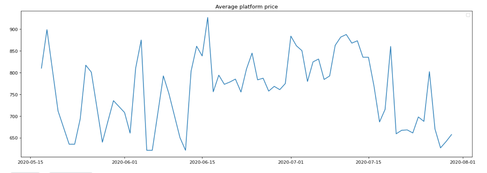
Price elasticity across the platform

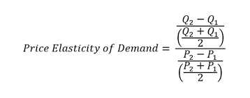
The average price of the platform has been changing drastically from time to time and this can only mean that demand is varying as well. But due to the unavailability of demand information, the price elasticity of demand cannot be calculated.

This plot provides a proxy for the GMV change(gross merchandising value) of the platform.

screenshot

Readers are encouraged to think about other hypotheses in support or against the problem statement which in turn will help in finding feasible solutions.  

5. Exploring Feasible Solutions

The problem statement states that identify independent price setters, and followers, the assumption being, the follower is following just one operator. We could be tempted to think, the follower could be checking multiple operators before setting the final price, just like users compare prices on Redbus, Makemystrip, Easemytrip before purchasing tickets.  This temptation is called conjunction fallacy! The probability of following one operator is higher than the probability of following two operators. Hence it’s safe to assume that comparing 1:1 operators pricing data and assigning setter and follower status is both heuristically as well as a statistically viable solution and the same has been followed in this solution.

How has the EDA helped with solutions?

1. On average 10% change in the initial and final price is strong evidence that operators are leveraging pricing to increase volumes.
2. The long-tailed wide bell curve for prices, hence the need to compare between similar buckets or similar price groups.
3. The majority of individual bus prices move along with the market prices. If this dint holds good, then it’s evidence of data anomaly or coding error.
4. On average buses list 30 days in advance giving operators enough time to mimic competitors pricing strategies.
5. 1:1 operator comparison to identify follower and setter, rather than 1:2 or otherwise, to avoid conjunction fallacy.

Follower Detection Algorithm V001:

1. Randomly select 2 bus id, B1 and B2 with P1 and P2 having sufficient data points.
2. Join the two datasets and keep relevant columns only.
3. The basic hypothesis is, the price change ratio(p’) will converge at some timestamp, meaning the prices have intersected, and there is a setter-follower behaviour.
4. Calculate the difference in price (~P )of wrt to P1 as well as P2. (P2-P1)/P1 and (P2-P1)/P2, assuming  B2 is the follower.
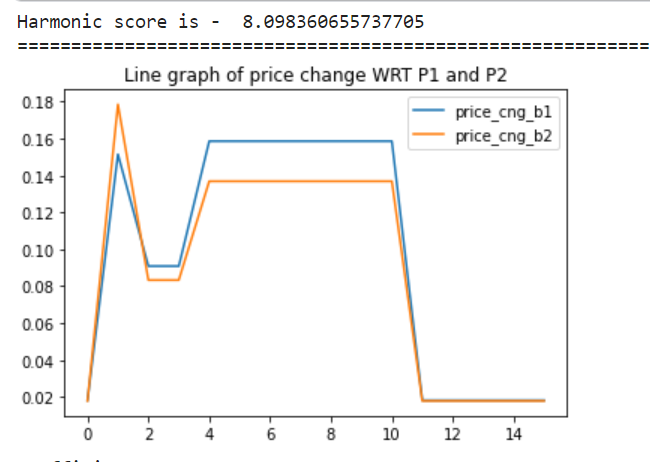
5. Get the average price change by calculating the harmonic mean of the ~p. (Different denominators P1 and P2, hence harmonic mean )
6. HM_Score = (max(hm) – min(hm))/ min(hm). If score is low, then less confidence in setter-follower relationship.
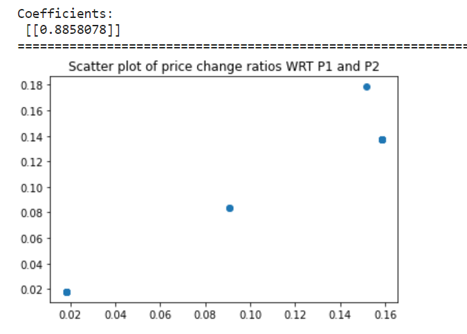
7.  The second aspect of the solution is to identify the coefficient(beta) of the equation ~P2 = C + beta*~P1. Ideally, the scatter plot will be at a slope of 45 degrees or have a positive correlation. And p-value of 0.8 to 1 is considered(experimental) good confidence.  And the intercept needs to be close to 0, meaning little or no difference in price, which could be convergence.
8. A combined score/metrics of p-value and hm_score can help identify a follower and a setter.
9. This is an initial, crude solution and can be further refined to improve its accuracy.

Code:

f = final_cleaned_df.copy()
b1 = f[(f["Bus"] == "a6951a59b64579edcf822ab9ea4c0c83") & (f["Service_Date"] == "15-07-2020 00:00")]
b2 = f[(f["Bus"] == "ab479dab4a9e6bc3eaefe77a09f027ed") & (f["Service_Date"] == "15-07-2020 00:00")]
recorded_dates_df = pd.concat([b1[["RecordedAt_new"]], b2[["RecordedAt_new"]]], axis = 0).drop_duplicates().sort_values(by = "RecordedAt_new").reset_index().drop(columns = "index")
joined_1  =  pd.merge(recorded_dates_df, b1, on=["RecordedAt_new"], how='left',suffixes=('_actuals', '_B1'))
joined_df =  pd.merge(joined_1, b2, on=["RecordedAt_new"], how='left',suffixes=('_B1', '_B2'))
joined_df
cols_to_keep = ["RecordedAt_new", "Service_Date_B1","Bus_B1","Bus_B2", "average_price_s1_s2_filled_B1", "average_price_s1_s2_filled_B2"]
model_df = joined_df[cols_to_keep]
model_df_2 = model_df.drop_duplicates()
## replace null of service date 
model_df_2['Service_Date_B1'] = model_df_2['Service_Date_B1'].fillna(model_df_2['Service_Date_B1'].value_counts().idxmax())
model_df_2['Bus_B1'] = model_df_2['Bus_B1'].fillna(model_df_2['Bus_B1'].value_counts().idxmax())
model_df_2['Bus_B1'] = model_df_2['Bus_B1'].fillna(model_df_2['Bus_B1'].value_counts().idxmax())
model_df_2.fillna(0, inplace = True)
test_a = model_df_2.sort_values(by = ["RecordedAt_new" ])
test_a = test_a[["Service_Date_B1","average_price_s1_s2_filled_B1" ]]
test_a["average_price_B1_new"] = test_a.groupby(["Service_Date_B1" ]).transform(lambda x: x.replace(to_replace=0, method='bfill'))
test_f = model_df_2.sort_values(by = ["RecordedAt_new" ])
test_f = test_f[["Service_Date_B1","average_price_s1_s2_filled_B2" ]]
test_f["average_price_B2_new"] = test_f.groupby(["Service_Date_B1" ]).transform(lambda x: x.replace(to_replace=0, method='bfill'))
model_df_2["average_price_B1_new"] = test_a["average_price_B1_new"] 
model_df_2["average_price_B2_new"] = test_f["average_price_B2_new"] 
model_df_3 = model_df_2[model_df_2["average_price_B1_new"] != 0][["average_price_B1_new","average_price_B2_new"] ]
from scipy.stats import hmean
## get the price change wrt to each bus price
model_df_2["price_cng_b1"] = abs(model_df_2.average_price_B1_new - model_df_2.average_price_B2_new)/model_df_2.average_price_B1_new 
model_df_2["price_cng_b2"] = abs(model_df_2.average_price_B1_new - model_df_2.average_price_B2_new)/model_df_2.average_price_B2_new 
model_df_2["harm_mean_price_cng"] = scipy.stats.hmean(model_df_2.iloc[:,8:10],axis=1)
model_df_2 = model_df_2[model_df_2["average_price_B1_new"] != 0]
model_df_2 = model_df_2[model_df_2["average_price_B2_new"] != 0]
model_df_2x = model_df_2.copy()
hm = scipy.stats.hmean(model_df_2x.iloc[:,8:10],axis=1)
display((max(hm) - min(hm))/ min(hm))
print("======================================================================================================")
model_df_3 = model_df_2[model_df_2["average_price_B1_new"] != 0][["price_cng_b1","price_cng_b2"] ]
model_df_3.plot();
plt.show()
# Create linear regression object
regr = linear_model.LinearRegression()
# Train the model using the training sets
# (X,Y)
regr.fit(np.array(model_df_2["price_cng_b1"]).reshape(-1,1),np.array(model_df_2["price_cng_b2"]).reshape(-1,1))
# The coefficients
print("Coefficients: n", regr.coef_)

6. Test For Accuracy and Evaluation

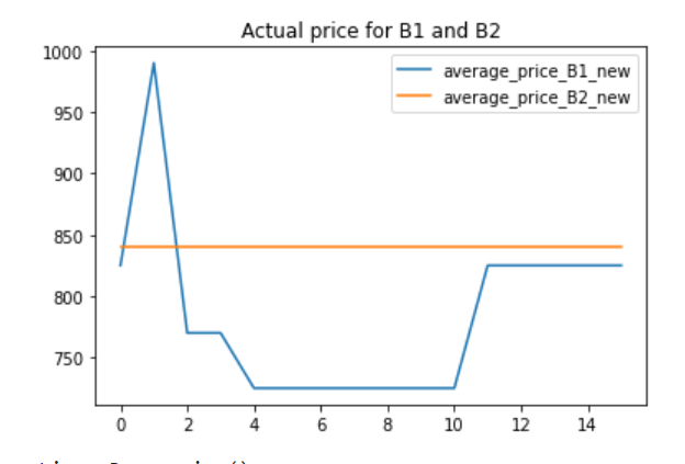
Manual evaluation B1 – 9656d6395d1f3a4497d0871a03366078 and B2 – 642c372f4c10a6c0039912b557aa8a22 and service date – 15-07-2020 00:00

Actual price data from 14 days time period. We see that B1 is a follower but with low confidence.

screenshot

The harmonic mean score((max(hm)-min(hm) )/ min(hm)) is high showing that the difference on average is about 8, meaning there is a significant difference in prices at some point in time.

screenshot

The co-efficient shows that (P2-P1)/P1 and (P2-P1)/P2 is linear, also a good R2 of above 75% would mean a healthy model as well. Intercept is close to 0 also supports our assumption.

Final confidence can be hm_score* coefficient = 8*0.8 = 6.4. This is absolute confidence. Relative confidence by normalizing across all combinations will provide a score between 0 and 1, which can be gauged more easily.

We can reject the null hypothesis and assume the alternate to be true.

While this isn’t an optimal solution, it’s a good reference point, to begin with. Smoothening the rough edges of the algorithm and refining it for accuracy will lead to better results.

Useful Resources and References

Data science can be broadly divided into business solution-centric and technology-centric divisions. The below resources will immensely help a business solution-centric data science enthusiast expand their knowledge.

1. Fixing cancellations in-cab market.
2. Don’t fall for the conjunction fallacy!
3. HBR – Managing Price, Gaining Profit
4. Pricing: Distributors’ most powerful value-creation lever
5. Ticket Sales Prediction and Dynamic Pricing Strategies in Public Transport
6. Pricing Strategies for Public Transport
7. The Pricing Is Right: Lessons from Top-Performing Consumer Companies
8. The untapped potential of a pricing strategy and how to get started
9. Kaggle notebook with the solution can be found on my Kaggle account.

End Notes

This article presents a preliminary, unitary method, to figure out fare setters and followers. The accuracy of preliminary methods tends to be questionable but sets a precedent for upcoming more resilient and curated methods. This methodology can be improved as well with more data points and features such as destination, boarding location, YOY comparisons, fleet size, passenger information etc. Moreover, anomaly detection modelling might provide more satisfactory results as well.

The dataset can also be used for price forecasting using ARIMA or deep learning methods such as LSTM etc.

Good luck! Here’s my Linkedin profile in case you want to connect with me or want to help improve the article. Feel free to ping me on Topmate/Mentro as well, you can drop me a message with your query. I’ll be happy to be connected. Check out my other articles on data science and analytics here.

The media shown in this article is not owned by Analytics Vidhya and are used at the Author’s discretion. 

Chrisx10 Dmello 15 Mar 2022

Data scientist! Extensively using data mining, data processing algorithms, visualization, statistics and predictive modelling to solve challenging business problems and generate insights.