Overview
Machine Learning is one of the most widely used concepts around the world. It will be essential in the healthcare sectors which will be useful for doctors to fasten the diagnosis. In this article, we will be dealing with the Heart disease dataset and will analyze, predict the result whether the patient has heart disease or normal, i.e. Heart disease prediction using Machine Learning. This prediction will make it faster and more efficient in healthcare sectors which will be a time-consuming process.
Key Takeaways
- This process involves data cleaning, data statistics, getting insights from the dataset.
- This involves four machine learning algorithms which will result in performance metrics of the model.
- The well-doing algorithm is implemented in the model and checking results with the real-time data.
This article was published as a part of the Data Science Blogathon.
Table of contents
Importing Libraries
import NumPy as np
import pandas as pd
import matplotlib.pyplot as plt
import seaborn as sns
import warnings
from sklearn.model_selection import KFold, StratifiedKFold, cross_val_score
from sklearn import linear_model, tree, ensemble
Reading the Data from CSV file
In this section, we will load and view the CSV file and its contents.
Filename: heart.csv
This dataset is sourced from the online repository of UCI.
Link: https://archive.ics.uci.edu/ml/datasets/Heart+Disease
Contents:
We have 14 attributes/features including target which will be age, gender, cholesterol level, exacting, chest pain, old peak, thalach, FBS, slope, thal, etc.
dataframe=pd.read_csv("/content/heart.csv")
data frame.head(10)
Output:
Inference: From the dataset, we have three types of data such as continuous, ordinal, and binary data.
Data Analysis
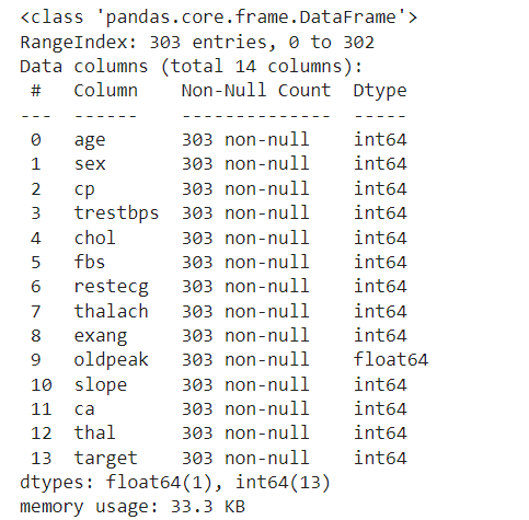
Let, we get some basic information about the dataset.
dataframe.info()
Output:
Now, let us look at whether the dataset has null values or not.
dataframe.isna().sum()
Output:
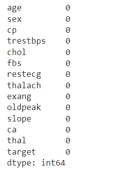
Inference: From this output, our data does not contain null values and duplicates. So, the data is good which will be further analyzed.
Correlation Matrix
Visulaizing the data features to find the correlation between them which will infer the important features.
plt.figure(figsize=(15,10))
sns.heatmap(dataframe.corr(),linewidth=.01,annot=True,cmap="winter")
plt.show()
plt.savefig('correlationfigure')
Output:
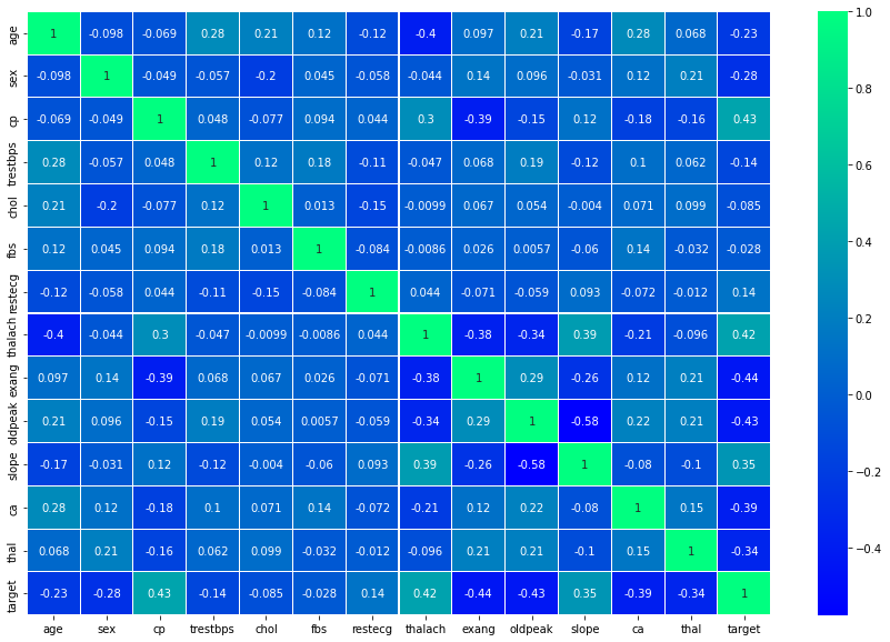
Inference:
From the above heatmap, we can understand that Chest pain(cp) and target have a positive correlation. It means that whose has a large risk of chest pain results in a greater chance to have heart disease. In addition to chest pain, thalach, slope, and resting have a positive correlation with the target.
Then, exercise-induced angina(exang) and the target have a negative correlation which means when we exercise, the heart requires more blood, but narrowed arteries slow down the blood flow. In addition to ca, old peak, thal have a negative correlation with the target.
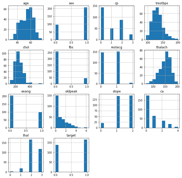
Let us see the relation between each features distribution with the help of histogram.
dataframe.hist(figsize=(12,12))
plt.savefig('featuresplot')
Output:
Train-Test Split
X_train, X_test,y_train, y_test=train_test_split(X,y,test_size=0.25,random_state=40)
We split the whole dataset into trainset and testset which contains 75% train and 25% test.
We can include this train set into classifiers to train our model and the test set is useful for predicting the performance of the model by different classifiers.
Algorithm Implementation
1 .Logistic Regression
from sklearn.model_selection import cross_val_score, GridSearchCV
from sklearn.linear_model import LogisticRegression
lr=LogisticRegression(C=1.0, class_weight='balanced', dual=False,
fit_intercept=True, intercept_scaling=1, l1_ratio=None,
max_iter=100, multi_class='auto', n_jobs=None, penalty='l2',
random_state=1234, solver='lbfgs', tol=0.0001, verbose=0,
warm_start=False)
model1=lr.fit(X_train,y_train)
prediction1=model1.predict(X_test)
from sklearn.metrics import confusion_matrix
cm=confusion_matrix(y_test,prediction1)
cm
sns.heatmap(cm, annot=True,cmap='winter',linewidths=0.3, linecolor='black',annot_kws={"size": 20})
TP=cm[0][0]
TN=cm[1][1]
FN=cm[1][0]
FP=cm[0][1]
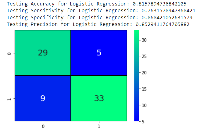
print('Testing Accuracy for Logistic Regression:',(TP+TN)/(TP+TN+FN+FP))
print('Testing Sensitivity for Logistic Regression:',(TP/(TP+FN)))
print('Testing Specificity for Logistic Regression:',(TN/(TN+FP)))
print('Testing Precision for Logistic Regression:',(TP/(TP+FP)))Output:
from sklearn.metrics import classification_report
print(classification_report(y_test, prediction1))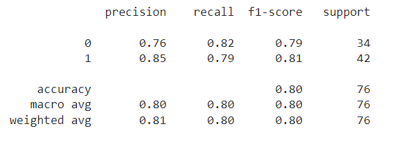
Inference: From the above report, we get the accuracy of the Logistic Regression classifier is about 80%.
2. Decision Tree
from sklearn.model_selection import RandomizedSearchCV
from sklearn.tree import DecisionTreeClassifier

tree_model = DecisionTreeClassifier(max_depth=5,criterion='entropy')
cv_scores = cross_val_score(tree_model, X, y, cv=10, scoring='accuracy')
m=tree_model.fit(X, y)
prediction=m.predict(X_test)
cm= confusion_matrix(y_test,prediction)
sns.heatmap(cm, annot=True,cmap='winter',linewidths=0.3, linecolor='black',annot_kws={"size": 20})
print(classification_report(y_test, prediction))

TP=cm[0][0]
TN=cm[1][1]
FN=cm[1][0]
FP=cm[0][1]
print('Testing Accuracy for Decision Tree:',(TP+TN)/(TP+TN+FN+FP))
print('Testing Sensitivity for Decision Tree:',(TP/(TP+FN)))
print('Testing Specificity for Decision Tree:',(TN/(TN+FP)))
print('Testing Precision for Decision Tree:',(TP/(TP+FP)))
Output:
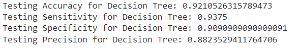
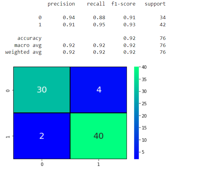
Inference: From the above report, we get the accuracy of the Decision Tree classifier is about 92%.
3. Random Forest Classifier
from sklearn.ensemble import RandomForestClassifier
rfc=RandomForestClassifier(n_estimators=500,criterion='entropy',max_depth=8,min_samples_split=5)
model3 = rfc.fit(X_train, y_train)
prediction3 = model3.predict(X_test)
cm3=confusion_matrix(y_test, prediction3)
sns.heatmap(cm3, annot=True,cmap='winter',linewidths=0.3, linecolor='black',annot_kws={"size": 20})
TP=cm3[0][0]
TN=cm3[1][1]
FN=cm3[1][0]
FP=cm3[0][1]
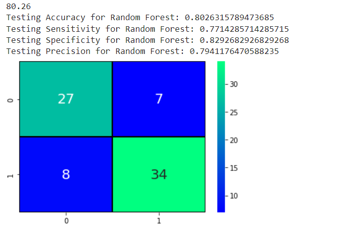
print(round(accuracy_score(prediction3,y_test)*100,2))
print('Testing Accuracy for Random Forest:',(TP+TN)/(TP+TN+FN+FP))
print('Testing Sensitivity for Random Forest:',(TP/(TP+FN)))
print('Testing Specificity for Random Forest:',(TN/(TN+FP)))
print('Testing Precision for Random Forest:',(TP/(TP+FP)))Output:
Let us see the classification report for Random Forest Classifier:
print(classification_report(y_test, prediction3))Output:
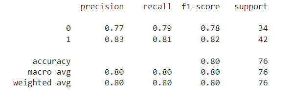
Inference: From the above report, we can get the accuracy of the Random Forest classifier is about 80%.
4. Support Vector Machines(SVM)
from sklearn.svm import SVC
svm=SVC(C=12,kernel='linear')
model4=svm.fit(X_train,y_train)
prediction4=model4.predict(X_test)
cm4= confusion_matrix(y_test,prediction4)
sns.heatmap(cm4, annot=True,cmap='winter',linewidths=0.3, linecolor='black',annot_kws={"size": 20})
TP=cm4[0][0]
TN=cm4[1][1]
FN=cm4[1][0]
FP=cm4[0][1]
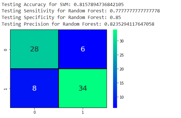
print('Testing Accuracy for SVM:',(TP+TN)/(TP+TN+FN+FP))
print('Testing Sensitivity for Random Forest:',(TP/(TP+FN)))
print('Testing Specificity for Random Forest:',(TN/(TN+FP)))
print('Testing Precision for Random Forest:',(TP/(TP+FP)))Output:
Let us see the classification report of SVM:
print(classification_report(y_test, prediction4))Output:
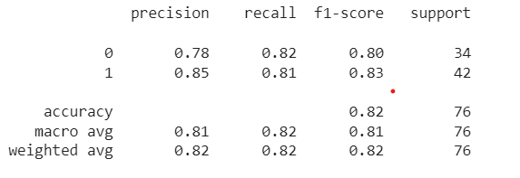
Inference: From the above report, we get the accuracy of the Support Vector Machine classifier is about 82%.
From the results that we got, as four machine learning algorithms like Logistic Regression, Random Forest, Support Vector Machines and Decision Trees. From the final results, we got Logistic Regression as 80%, Random Forest as 80%, Support Vector Machines as 82%, and Decision Trees as 92%. We can conclude that the Decision Tree algorithm is the best algorithm for our model with the highest accuracy around 92 percent.
Final Model Implementation
Now, we can apply the best working algorithm (i.e., Decision Tree Classifier) into our model and check whether our model will result in the correct output or not with the help of available data.
CASE 1 – For Heart Disease data
input=(63,3,145,233,150,2.3,0)
input_as_numpy=np.asarray(input)
input_reshaped=input_as_numpy.reshape(1,-1)
pre1=tree_model.predict(input_reshaped)
if(pre1==1):
  print("The patient seems to be have heart disease:(")
else:
  print("The patient seems to be Normal:)")
Output:

CASE 2 – For Normal Data
input=(72,1,125,200,150,1.3,1)
input_as_numpy=np.asarray(input)
input_reshaped=input_as_numpy.reshape(1,-1)
pre1=tree_model.predict(input_reshaped)
if(pre1==1):
  print("The patient seems to be have heart disease:(")
else:
  print("The patient seems to be Normal:)")
Output:

Conclusion
Finally, we can conclude that real-time predictors will be essential in the healthcare sector nowadays. From this project, we will be able to predict real-time heart disease using the patient’s data from the model using the Decision Tree Algorithm, thereby making accurate heart disease prediction using machine learning. I hope that you are all excited about the blog. Let us know your thoughts in the comments!
Frequently Asked Questions
Q1. What is the role of machine learning in heart disease?
A. Machine learning plays a crucial role in heart disease by enabling early detection, accurate diagnosis, and personalized treatment. It can analyze large amounts of patient data, including medical records, imaging tests, and genetic information, to identify patterns and predict the risk of developing heart disease. Machine learning algorithms can also assist in identifying specific heart conditions, such as arrhythmias, based on ECG data. Moreover, they aid in developing personalized treatment plans by considering individual patient characteristics and response to therapies. By leveraging machine learning, healthcare professionals can improve patient outcomes, optimize resource allocation, and enhance overall cardiac care.
Q2. What algorithm is used for heart disease prediction?
A. There are several machine learning algorithms used for heart disease prediction, including logistic regression, decision trees, random forests, support vector machines (SVM), and artificial neural networks. Each algorithm has its strengths and limitations, and the choice depends on the specific dataset and problem at hand. Ensemble methods, such as random forests, are often favoured for their ability to combine multiple algorithms and improve prediction accuracy.
Q3. how machine learning is used in heart disease prediction?
Machine learning algorithms, fed with vast patient data, effectively predict heart disease risk, enabling personalized medicine and improved healthcare outcomes.
Thanks for reading the article!
The media shown in this article is not owned by Analytics Vidhya and are used at the Author’s discretion.


