Deploying a Keras Flower Classification Model with Gradio

This article was published as a part of the Data Science Blogathon.

Background on Flower Classification Model

Deep learning models, especially CNN (Convolutional Neural Networks), are implemented to classify different objects with the help of labeled images. The models are trained with these images to great accuracy, tested, and then deployed for performance. For example, a trained image classification model accepts images of cars and identifies the brand or the make of the car, such as Tata, Maruti Suzuki, BMW, Mercedes, etc. In the same way, these models can also be trained to classify other objects too. Pre-trained models like VGG16, VGG19, ResNet, etc., can be used in
transfer learning to classify different objects with minimal code.

Introduction to Flower Classification

In the same context, flower images are always pleasant to look at. We find a variety of attractive flowers in nature with different shapes and enchanting colors. At times, we see a flower we like but cannot identify. Computer vision can help us correctly identify the flower species in such a situation. A web app accessed on a browser using a phone or a laptop can accept the flower image and perform predictions to identify the flower image. In fact, such apps built with deep learning can prove immensely beneficial in agriculture and horticulture domains.

Image classification is an important part of computer vision with applications in automotive, agriculture, healthcare, transportation & logistics, traffic management, space research, and many more.

In this tutorial, we will demonstrate how to easily build an image classification model using Keras and deploy it using Gradio. This image classification model will be trained to classify images of different flowers.

Building a Flower Image Classifier using Keras

We will import all the required libraries and packages:

import matplotlib.pyplot as plt
import numpy as np
import os
import PIL

import tensorflow as tf
from tensorflow import keras
from tensorflow.keras import layers
from tensorflow.keras.models import Sequential

Next, we will download the flower dataset from TensorFlow. The dataset can be downloaded from here.

import pathlib
dataset_url = "https://storage.googleapis.com/download.tensorflow.org/example_images/flower_photos.tgz"

To obtain and extract the data, we’ll use the untar data function, which will automatically download and untar the dataset.

data_dir = tf.keras.utils.get_file('flower_photos', origin=dataset_url, untar=True)
data_dir = pathlib.Path(data_dir)

We now have a copy of the dataset available after downloading it. Let’s use the following command to see how many images are there:

image_count = len(list(data_dir.glob('*/*.jpg')))
print(image_count)

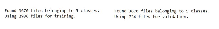
The dataset includes 3670 images of flowers organized into five subdirectories: dandelion, roses, tulips, daisy, and sunflowers. The following command can be used to display the subdirectories:

print(os.listdir(data_dir))

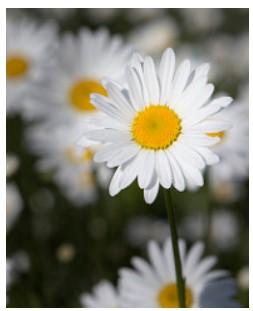
Then, we’ll run the following command to see some images from the roses and daisy subdirectories.

roses = list(data_dir.glob('roses/*'))
PIL.Image.open(str(roses[1]))

daisy = list(data_dir.glob('daisy/*'))
PIL.Image.open(str(daisy[2]))

We resize the images in our dataset because they are of different sizes. We specify the image height and width to do this. We also specify the batch size, which is the number of images used by the model during each epoch.

batch_size = 32
img_height = 180
img_width = 180

We are now using the image dataset by calling the directory() function to read and resize the images in the database. We’re also dividing the images in an 80:20 ratio for classification. The training ratio is 0.8, whereas the validation ratio is 0.2.

train_ds = tf.keras.utils.image_dataset_from_directory(
  data_dir,
  validation_split=0.2,
  subset="training",
  seed=123,
  image_size=(img_height, img_width),
  batch_size=batch_size)

Similarly, we are calling the directory() function to read the validation images from the directory.

val_ds = tf.keras.utils.image_dataset_from_directory(
  data_dir,
  validation_split=0.2,
  subset="validation",
  seed=123,
  image_size=(img_height, img_width),
  batch_size=batch_size)

Therefore, out of the total 3670 image files belonging to 5 classes, we are using 2936 image files for training and 734 image files for validation.

The class names can be found in the class names property of these datasets. In alphabetical order, they correspond to the directory names.

class_names = train_ds.class_names
print(class_names)

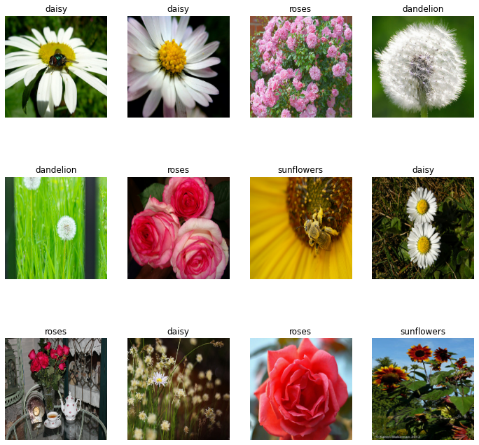
We can also print a few sample images from the training dataset using the following code –

import matplotlib.pyplot as plt
plt.figure(figsize=(12, 12))
for images, labels in train_ds.take(1):
  for i in range(12):
    ax = plt.subplot(3, 4, i + 1)
    plt.imshow(images[i].numpy().astype("uint8"))
    plt.title(class_names[labels[i]])
    plt.axis("off")

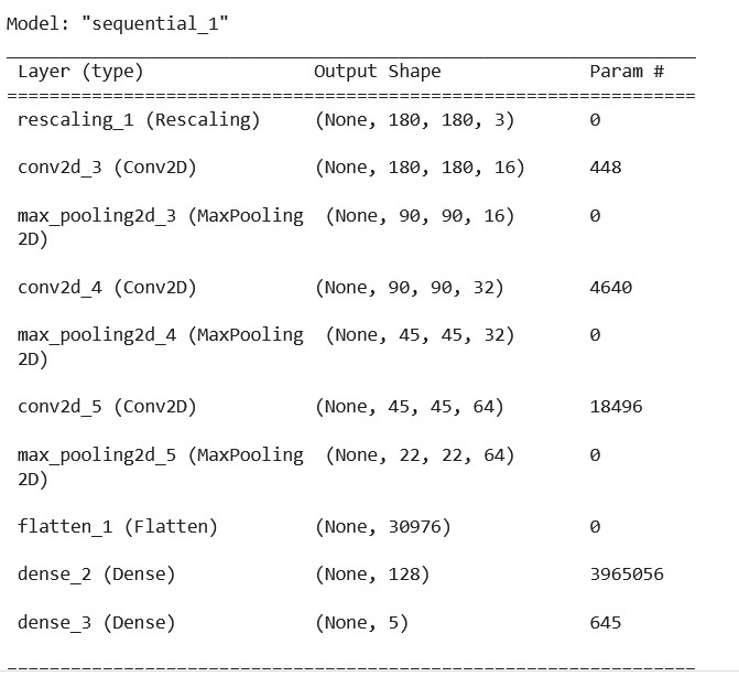
Now we’ll create the Sequential model, which is made up of three convolution blocks, each with a max-pooling layer. A ReLU activation function is used to activate a fully connected layer with 128 units on top of it. In addition, the RGB channel values are between [0, 255]. This isn’t ideal for a neural network; we’ll use the Rescaling function to normalize values.

Now we’ll use the following code to build the model

num_classes = len(class_names)

model = Sequential([
  layers.experimental.preprocessing.Rescaling(1./255, input_shape=(img_height, img_width, 3)),
  layers.Conv2D(16, 3, padding='same', activation='relu'),
  layers.MaxPooling2D(),
  layers.Conv2D(32, 3, padding='same', activation='relu'),
  layers.MaxPooling2D(),
  layers.Conv2D(64, 3, padding='same', activation='relu'),
  layers.MaxPooling2D(),
  layers.Flatten(),
  layers.Dense(128, activation='relu'),
  layers.Dense(num_classes,activation='softmax')
])

model.compile(optimizer='adam',
              loss=tf.keras.losses.SparseCategoricalCrossentropy(from_logits=True),
              metrics=['accuracy'])

The following parameters are important to compile function:

• optimizer – We chose Adam as the optimizer. It will increase and improve the convolution neural network’s performance. It also manages any training errors that the CNN may have.

• loss – This is the function that collects all the errors that the CNN experiences while training. Because the image dataset has various classes, we apply SparseCategoricalCrossentropy (five classes).

• metrics – This function calculates the total CNN accuracy score after training. We set its value to accuracy.

We can view all the layers of the network using the ‘model.summary’ function:

model.summary()

Next, we fit the model on the training_images and the validation_images. The convolution neural network will learn from training images to perform image classification. We are also setting the number of epochs to 15.

epochs=15
history = model.fit(
  train_ds,
  validation_data=val_ds,
  epochs=epochs
)

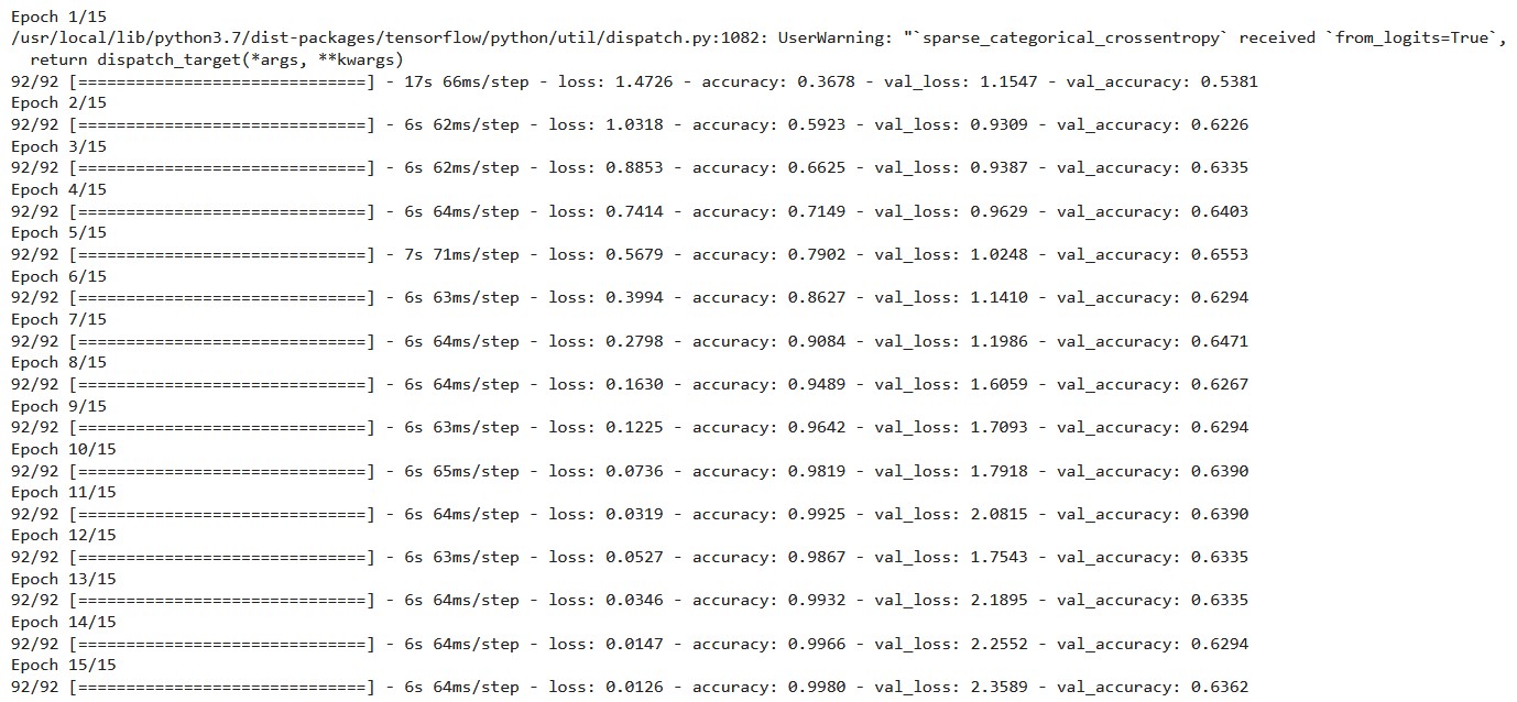
During each epoch, the output displays the CNN loss, training accuracy, and validation accuracy score. The initial training loss score is 1.4726, and the final training loss score is 0.0126. It shows that CNN errors have decreased over time.

The initial training accuracy score is 0.3678, and the final accuracy score is 0.9980. It illustrates that as the number of epochs increased, CNN’s performance improved. The value of validation accuracy rises from 0.5381 to 0.6362.

We can plot the loss and model accuracy on the training and validation sets to visualize the training results.

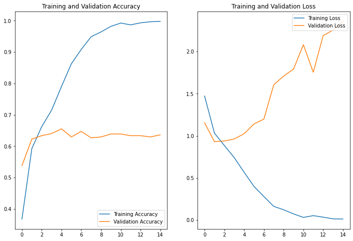
Since we have only trained the model for 15 epochs, the final validation accuracy score is ~64%. The model accuracy can further be improved by modifying the CNN layers, such as adding dropout layers, increasing the number of layers, and implementing data augmentation to increase the size of the dataset. For demo purposes, we can use the model as it is for deploying it as a web app.

Next, we’ll use the predict input image function. For the function to work, the input image takes four dimensions, as seen in the code below. To convert the input image to four dimensions, the function will use the img.reshape method. The input image will then be classified using model.predict function.

def predict_input_image(img):
  img_4d=img.reshape(-1,180,180,3)
  prediction=model.predict(img_4d)[0]
  return {class_names[i]: float(prediction[i]) for i in range(5)}

The function then produces a dictionary containing each predicted class and its associated probability. The most likely class will be the right prediction or classification.

Gradio can now be used to add a user interface for interacting with our trained CNN.

Deploying the Deep Learning Model Using Gradio

Gradio is a machine learning library that transforms your trained machine learning model into an interactive application. Gradio provides simple user interfaces (UI) that enable users to interact with a trained machine learning model. It generates a web interface via which the user can test the trained model and view the prediction results. Gradio’s user interface can be simply integrated straight into the Python notebook (either Jupyter notebook or Google Colab notebook) without the need to install any dependencies. Gradio interacts directly with popular machine learning libraries such as Sckit-learn, Tensorflow, Keras, PyTorch, and Hugging Face Transformers.

Let’s start by installing the gradio library:

!pip install gradio

Now we will import the Gradio package.

import gradio as gr

Before creating Gradio’s user interface, we must specify the size of the picture that Gradio’s input component will store. As shown in the code below, we are also providing the number of labeled classes in the image dataset.

image = gr.inputs.Image(shape=(180,180))
label = gr.outputs.Label(num_top_classes=5)

gr.Interface(fn=predict_input_image, inputs=image, outputs=label,interpretation='default').launch(debug='True')

The output of running the code will provide a URL for your Gradio app. This link for the app expires after 72 hours.

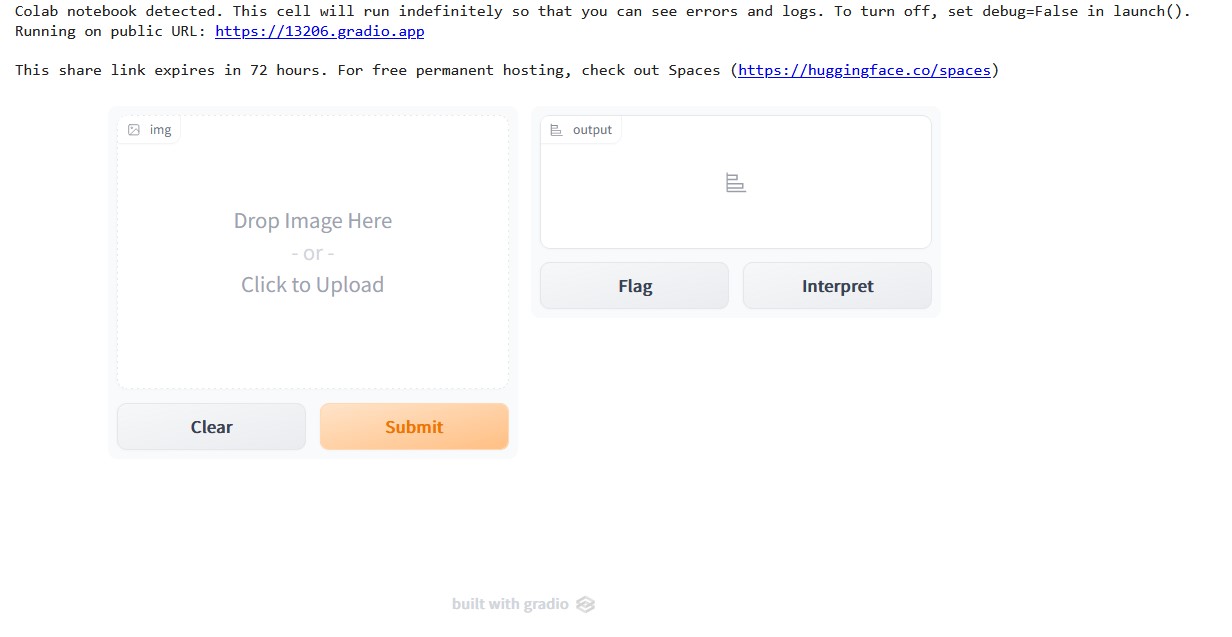
The given link will launch a new browser window. The newly opened tab displays the GradioUI. We can place the image there or submit the image to be classified using the GradioUI. Let us upload an image.

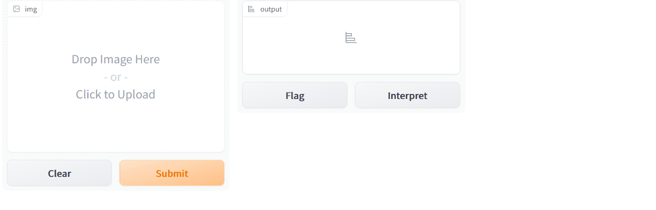
The image that was uploaded is shown in the output above. We then press the Submit button to get the classification results. We get the result after hitting the submit button.

This indicates that we have successfully deployed our app on the web using Gradio.

Conclusion

In this tutorial, we learned how to build an image classifier using Keras and deploy it using Gradio.

Here are some key takeaways from this article-

• Deep learning techniques can be used for building image classifiers for various types of flower images. We built a simple deep learning model to classify five types of flowers – roses, daisy, dandelion, tulips, and sunflowers.
• A similar approach can be used to build image classifiers for plants or leaf images. Such models are in demand and applicable in the agriculture domain.
• It is easier to set up an image classification model in Tensorflow using the Keras API.
• The developed image learning model can be deployed with minimal lines of code using Gradio.
• Using Gradio, we can add a simple GUI to our model to interact with the model and deploy it as a web app.

I hope you found the article interesting. Feel free to build an image classifier of your choice and deploy it on Gradio using the steps mentioned in this article. You can find the complete code for this tutorial on my GitHub repository.

The media shown in this article is not owned by Analytics Vidhya and is used at the Author’s discretion.