A Simple Image Classification Project To Kickstart your Deep Learning Journey!

This article was published as a part of the Data Science Blogathon

Introduction

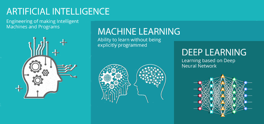
Before starting, we first need to understand what Deep Learning is. We all understand that Artificial Intelligence is a vast ocean with multiple subsets and one of them is Machine Learning and Deep Learning is a subset that falls under the topic of Machine Learning. We can describe Machine Learning as making the computer system act independently without too much human intervention, while Deep Learning is allowing the computers to think by stimulating a model inspired by the human brain. This is modelled by Neural Networks.

Image Classification with Deep Learning

In this article, we will understand the basics of Deep Learning by deploying a neural network that aims to classify flower images on MATLAB. This is a great tool that uses a proprietary multi-paradigm programming language and a numeric computing environment. So let’s get started!

Classify Images

We will first import the images that are in our library using the following commands.

img1 = imread("file01.jpg");
imshow(img1)

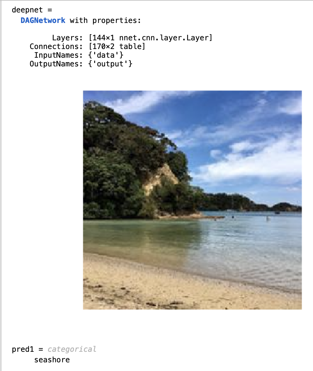
Next, we will load a predefined network called GoogLeNet, which you can try out with other pertained networks too. We will make use of this pertained network that can classify various types of objects like cars, beaches, cupcakes, and more.

deepnet = googlenet
pred1 = classify(deepnet,img1)

This show successfully imports an image and classifies it accordingly. The following is my output:

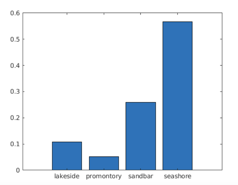
We can check the prediction scores by first collecting the prediction scores and then extracting the ones that have a higher threshold than others. And finally, making a bar chart with labels can help us visualize the classification process.

[pred,scores] = classify(deepnet,img)
highscores = scores > 0.01;
bar(scores(highscores))
xticklabels(categorynames(highscores))

 

Now let’s understand how this is happening. 

The GoogLeNet is a Convolutional Neural Network, it has layers that process features and data of the image. The layers included are Convolutional, ReLU, Pooling, Fully Connected, and Classification Output.

The convolutional layers in a neural network will be the first layer to extract features from an input image. It will summarize the presence of features in an input image, while the pooling layers provide an approach to downsampling feature maps by summarizing the presence of features in patches of the feature map. It helps in compressing the number of parameters to learn and the amount of computation performed in the network (Brownlee, 2019).

Next, the ReLU layers will normalize the data by returning 0 if any negative input is perceived. Subsequently, the fully connected layer will connect the layers and compile the data extracted by previous layers to form the final output. And lastly, the output layer will finally give the prediction strength for each category, and the image will be classified as the label with the highest confidence level. The network is trained by carrying out this on large sets of training data to learn the correct behaviour of the model.

Preprocessing Images for Classification

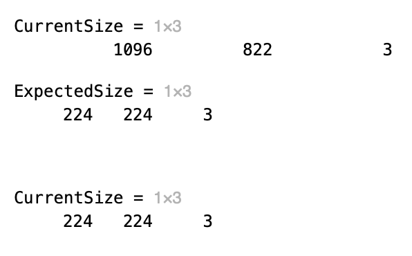
Sometimes the input images may vary in size or colour. It is the job of preprocessing to covert these images into a standard size and colour scale for classification. We need all images to be of the same standard to make the processing easier.

We first check the current size of the image, then we will check what is the expected size of the neural network. And we will resize the image accordingly.

CurrentSzie = size(img)
deepnet = googlenet;
inlayer = deepnet.Layers(1)
ExpectedSize = inlayer.InputSize
img = imresize(img,[224 224]);
imshow(img)

Transfer Learning

Now we will start customizing the network to meet our expectation of classifying a flower. In the previous sections we used the pertained network as is, this will work to classify the images that it has been trained with. But if we want to classify a variety of flowers, the network will not be able to do this as it has not been trained with the training set specific to flowers, hence we will modify the GoogLeNet to fit the problem and train it with the flower training set. The process of customizing a pertained network via modification and retaining with new data set is called Transfer Learning.

To perform transfer learning, we will need to create three components:

1. An array of layers representing the deep neural network. For transfer learning, this is created by modifying a preexisting network, in our case this is GoogLeNet.
2. A training set. This will include images with known labels to be used as training data.
3. A variable containing the options that control the behaviour of the training algorithm, for instance, learning rate, batch size, etc.

We will first load the image set that is to be used for training and testing purposes. Then we will extract the label name from the files loaded and save these for further usage. Next, we need to split the images loaded into the system into two sectors: one for training and another for testing. Here we will keep 60% of the images for the training set and the remaining 40% will be used as the testing set.

load pathToImages
flwrds = imageDatastore(pathToImages,"IncludeSubfolders",true);
flowernames = flwrds.Labels
flwrds = imageDatastore(pathToImages,"IncludeSubfolders",true,"LabelSource","foldernames")
flowernames = flwrds.Labels
[flwrTrain,flwrTest] = splitEachLabel(flwrds,0.6)

Modifying Network Layers

To modify GoogLeNet’s architecture, we will first need to extract the layer graph. Then to customize the network, we will first replace the fully connected layer. This is done by creating a new layer with only the number of neurons that we require. We will name this “fc” with 12 neurons.

lgraph = layerGraph(deepnet)
fc = fullyConnectedLayer(12,"Name","new_fc")

Next, we will modify individual elements of a layer graph. We will first replace the last fully connected layer of the network with the new fully connected layer that we created: “fc”. And then we will change the output layer. Currently, the output layer will contain the labels that are originally in the GoogLeNet, these labels will not be required in classifying the flowers. So, we will create a black output layer, and the 12 label classes will be fed into this layer during the training phase.

lgraph = replaceLayer(lgraph,"loss3-classifier",fc)
out = classificationLayer("Name","new_out")
lgraph = replaceLayer(lgraph,"output",out)

Set Training Options

We will set the training options to the default option of “stochastic gradient descent with momentum”, while only changing the Initial Learn Rate to a smaller value: 0.01.

This Initial Learn Rate will control how well the neural network algorithm changes the network weights. Since we are modifying an existing network, we need to change the weights less aggressively when compared to training a network from scratch.

opts = trainingOptions("sgdm","InitialLearnRate",0.001)

Train network

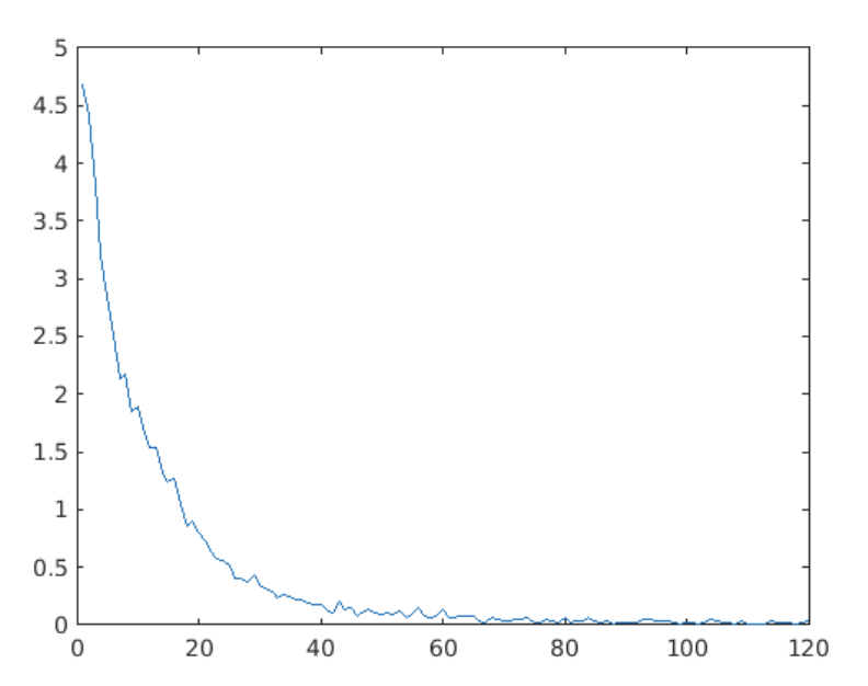
Now that we have customized the features of the network, we can train it with the training flower image set. We can run the network and plot the graph to see how the training is perceived by the network. We need the network to be trained well, and we should be able to see a decreasing training loss. This means that the more the network is training, the fewer classification errors are being made. This is a positive result for us.

[flowernet,info] = trainNetwork(flwrTrain, lgraph, options);
plot(info.TrainingLoss)

Classify images with trained network

testpreds = classify(flowernet,flwrTest);

fname = testImgs.Files

img1 = imread ("/CourseData/Flowers224/crocus/image_0399.jpg");

imshow(img1)

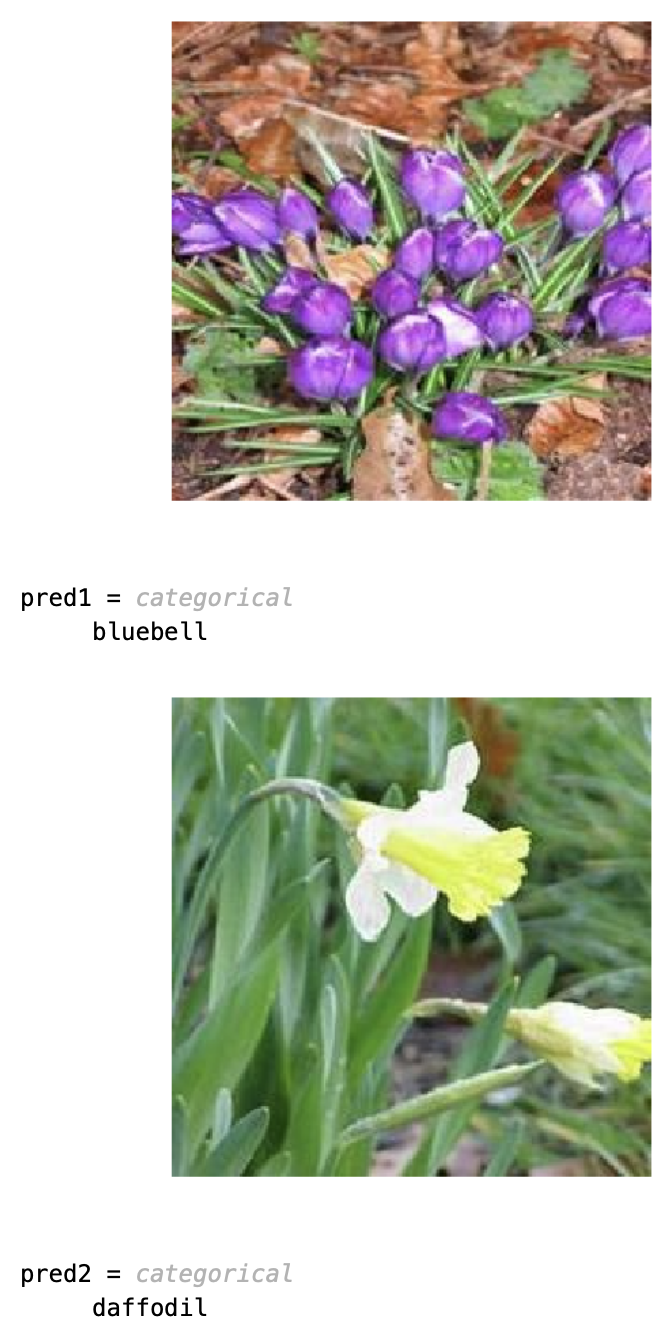
pred1 = classify(flowernet, img1)

img2 = imread("/CourseData/Flowers224/daffodil/image_0079.jpg");

imshow(img2)

pred2 = classify(flowernet, img2)

We can now use the trained network to classify the flower images that were loaded in the starting. I also did the classification of two individual flower images to check the predictions of those flowers.

Evaluate Performance

Performance evaluation is necessary to understand how effective the network is, we need to get the accuracy and training loss experienced.

Loss and accuracy give overall measures of the network’s performance. It can be particularly informative to understand how the network is performing to different types of images. We can calculate and displays the confusion matrix for the predicted classifications. The element of the confusion matrix gives a count of how many images from the network are predicted accurately. The diagonal elements represent correct classifications; off-diagonal elements represent misclassifications.

Firstly, we need to determine how many of the test images the network correctly classified by comparing the predicted classification with the known classification. For this, we extract the actual labels from the image files. They do a logical comparison with the actual labels and the predicted label outputs to get a count of how many were correctly classified. After this, we calculate the fraction of test images correctly classified by dividing by the total number of test images. And then finally compute the confusion matrix to determine the rate of classification and misclassification.

flwrActual = flwrTest.Labels;
numCorrect = nnz(flwrPreds == flwrActual)
fracCorrect = numCorrect/numel(flwrPreds)
confusionchart(flwrTest.Labels,flwrPreds)

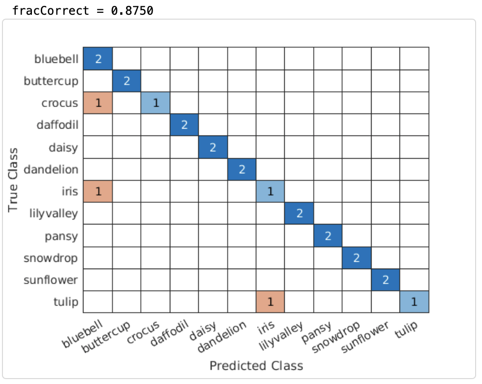
As we can see that the number of misclassifications is minimal compared to the accurate predictions. In order to further reduce the amount of misclassification, we can train the network more with a variety of flower images.

With that, we come to the end of this project. Hope you have understood the basics of Deep Learning and were successfully able to implement the image classification of flowers. This is a vast ocean, and you can find multiple projects and ideas out there that have further deeper your knowledge and understanding of the concept of Deep Learning.

References:

Brownlee, J. 2019. A Gentle Introduction to Pooling Layers for Convolutional Neural Networks [online] Machine Learning Mastery. Available at: <https://machinelearningmastery.com/pooling-layers-for-convolutional-neural-networks/> [Accessed 14 July 2021]

About the Author

Saniya is a final year Computer Science student studying at the University of Wollongong Dubai. She harbours a deep interest in Artificial Intelligence and Data Science. Check out her LinkedIn here.