Time Series Forecasting Using Python

This article was published as a part of the Data Science Blogathon.

Introduction on Time Series Forecasting Python

Unicorn Investors wants to make an investment in a new form of transportation – JetRail. JetRail uses Jet propulsion technology to run rails and move people at a high speed! The investment would only make sense if they can get more than 1 Million monthly users within the next 18 months. In order to help Unicorn Ventures in their decision, you need to forecast the traffic on JetRail for the next 7 months. You are provided with traffic data of JetRail since inception in the test file.

You can get the dataset here 

It is advised to look at the dataset after completing the hypothesis generation part.

Let’s Understand, What is Time Series Data?

Which of the following do you think is an example of time series? Even if you don’t know, try making a guess.

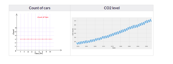
Time Series is generally data that is collected over time and is dependent on it. Here we see that the count of cars is independent of time, hence it is not a time series. While the CO2 level increases with respect to time, hence it is a time series.

Let us now look at the formal definition of Time Series.

A series of data points collected in time order is known as a time series. Most business houses work on time series data to analyze sales numbers for the next year, website traffic, count of traffic, the number of calls received, etc. Data of a time series can be used for forecasting.

Not every data collected with respect to time represents a time series. Some of the examples of time series prediction Python are:

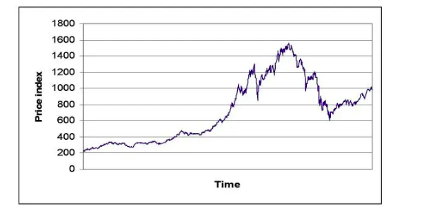
Stock Price

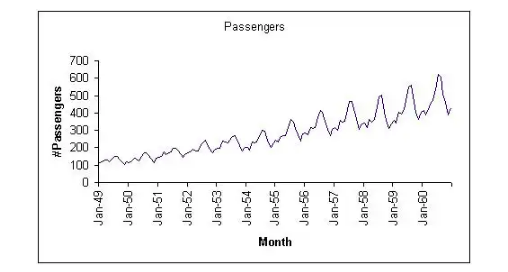
Passenger Count of Airlines

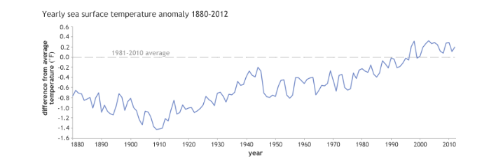
Temperature Over Time

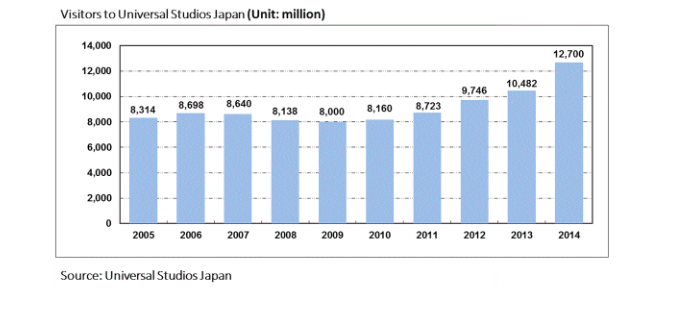
A Number of Visitors in a Hotel

Now that we can differentiate between a Time Series and a non-Time Series data. let us explore Time Series further.

Now as we have an understanding of what a time series is and the difference between a time series and a non-time series, let’s now look at the components of a time series.

Components of a Time Series Forecasting in Python

1. Trend

A trend is a general direction in which something is developing or changing. So we see an increasing trend in this time series. We can see that the passenger count is increasing with the number of years. Let’s visualize the trend of a time series:

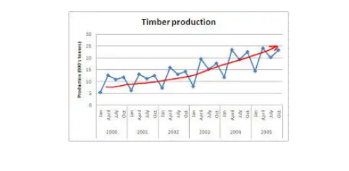
Example

Here the red line represents an increasing trend of the time series.

2. Seasonality

Another clear pattern can also be seen in the above time series, i.e., the pattern is repeating at a regular time interval which is known as the seasonality. Any predictable change or pattern in a time series that recurs or repeats over a specific time period can be said to be seasonality. Let’s visualize the seasonality of the time series:

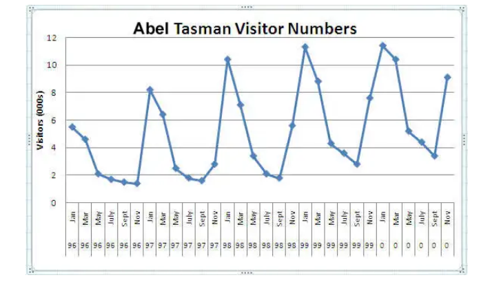
Example

We can see that the time series is repeating its pattern after every 12 months i.e there is a peak every year during the month of January and a trough every year in the month of September, hence this time series has a seasonality of 12 months.

Difference Between a Time Series and Regression Problem

Here you might think that as the target variable is numerical it can be predicted using regression techniques, but a time series problem is different from a regression problem in the following ways:

• The main difference is that a time series is time-dependent. So the basic assumption of a linear regression model that the observations are independent doesn’t hold in this case.
• Along with an increasing or decreasing trend, most Time Series have some form of seasonality trends,i.e. variations specific to a particular time frame.

So, predicting a time series using regression techniques is not a good approach.

Time series analysis comprises methods for analyzing time-series data in order to extract meaningful statistics and other characteristics of the data. Time series forecasting is the use of a model to predict future values based on previously observed values.

Understanding the Data

We will start with the first step, i.e Hypothesis Generation. Hypothesis Generation is the process of listing out all the possible factors that can affect the outcome.

Hypothesis generation is done before having a look at the data in order to avoid any bias that may result after the observation.

1) Hypothesis Generation

Hypothesis generation helps us to point out the factors which might affect our dependent variable. Below are some of the hypotheses which I think can affect the passenger count(dependent variable for this time series problem) on the JetRail:

There will be an increase in traffic as the years pass by.

• Explanation – Population has a general upward trend with time, so I can expect more people to travel by JetRail. Also, generally, companies expand their businesses over time leading to more customers traveling through JetRail.

The Traffic will be High from May to October

• Explanation – Tourist visits generally increase during this time period.

Traffic on Weekdays will be More as Compared to Weekends/Holidays.

• Explanation – People will go to the office on weekdays and hence the traffic will be more

Traffic during the Peak Hours will be High.

• Explanation – People will travel to work and college.

We will try to validate each of these hypothesis based on the dataset. Now let’s have a look at the dataset.

After making our hypothesis, we will try to validate them. Before that, we will import all the necessary packages.

2) Getting the System Ready and Loading the Data

Versions:

• Python = 3.7
• Pandas = 0.20.3
• sklearn = 0.19.1

Now we will import all the packages which will be used throughout the notebook.

import pandas as pd 
import numpy as np          # For mathematical calculations 
import matplotlib.pyplot as plt  # For plotting graphs 
from datetime import datetime    # To access datetime 
from pandas import Series        # To work on series 
%matplotlib inline 
import warnings                   # To ignore the warnings
warnings.filterwarnings("ignore")

Now let’s read the train and test data

Python Code:

Let’s make a copy of the train and test data so that even if we do changes in these datasets we do not lose the original dataset.

train_original=train.copy()
test_original=test.copy()

After loading the data, let’s have a quick look at the dataset to know our data better.

3) Dataset Structure and Content

Let’s dive deeper and have a look at the dataset. First of all, let’s have a look at the features in the train and test dataset.

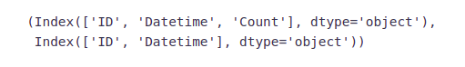
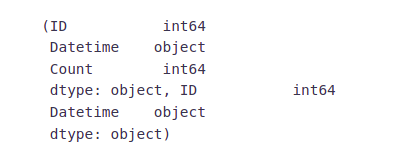
train.columns, test.columns

We have ID, Datetime, and the corresponding count of passengers in the training file. For the test file we have ID and Datetime only so we have to predict the Count for the test file.

Let’s understand each feature first:

• ID is the unique number given to each observation point.
• Datetime is the time of each observation.
• The count is the passenger count corresponding to each Datetime.

Let’s look at the data types of each feature.

train.dtypes, test.dtypes

• ID and Count are in integer format while the Datetime is in object format for the training file.
• ID is in integer and Datetime is in object format for the test file.

Now we will see the shape of the dataset.

train.shape, test.shape

We have 18288 different records for the Count of passengers in the train set and 5112 in the test set.

Now we will extract more features to validate our hypothesis.

4) Feature Extraction

We will extract the time and date from the Datetime. We have seen earlier that the data type of Datetime is an object. So first of all we have to change the data type to DateTime format otherwise we can not extract features from it.

train['Datetime'] = pd.to_datetime(train.Datetime,format='%d-%m-%Y %H:%M') 
test['Datetime'] = pd.to_datetime(test.Datetime,format='%d-%m-%Y %H:%M') 
test_original['Datetime'] = pd.to_datetime(test_original.Datetime,format='%d-%m-%Y %H:%M') 
train_original['Datetime'] = pd.to_datetime(train_original.Datetime,format='%d-%m-%Y %H:%M')

We made some hypothesis for the effect of the hour, day, month, and year on the passenger count. So, let’s extract the year, month, day, and hour from the Datetime to validate our hypothesis.

for i in (train, test, test_original, train_original):
    i['year']=i.Datetime.dt.year 
    i['month']=i.Datetime.dt.month 
    i['day']=i.Datetime.dt.day    
    i['Hour']=i.Datetime.dt.hour

We made a hypothesis for the traffic pattern on weekdays and weekends as well. So, let’s make a weekend variable to visualize the impact of weekends on traffic.

• We will first extract the day of the week from Datetime and then based on the values we will assign whether the day is a weekend or not.
• Values of 5 and 6 represents that the days are weekend.

• train[‘day of week’]=train[‘Datetime’].dt.dayofweek
• temp = train[‘Datetime’]

Let’s assign 1 if the day of the week is a weekend and 0 if the day of the week in not a weekend.

def applyer(row):
    if row.dayofweek == 5 or row.dayofweek == 6:

        return 1

    else:

        return 0

temp2 = train['Datetime'].apply(applyer) 
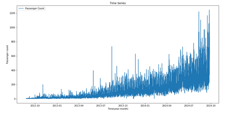
train['weekend']=temp2

Let’s look at the time series.

train.index = train['Datetime'] 
df=train.drop('ID',1) 
ts = df['Count'] 
plt.figure(figsize=(16,8)) 
plt.plot(ts, label='Passenger Count') 
plt.title('Time Series') 
plt.xlabel("Time(year-month)") 
plt.ylabel("Passenger count") 
plt.legend(loc='best')

Here we can infer that there is an increasing trend in the series, i.e., the number of counts is increasing with respect to time. We can also see that at certain points there is a sudden increase in the number of counts. The possible reason behind this could be that on a particular day, due to some event the traffic was high.

We will work on the training file for all the analysis and will use the test file for forecasting.

Let’s recall the hypothesis that we made earlier:

• Traffic will increase as the years pass by
• Traffic will be high from May to October
• Traffic on weekdays will be more
• Traffic during the peak hours will be high

After looking at the dataset, we will now try to validate our hypothesis and make other inferences from the dataset.

5) Exploratory Analysis

Let us try to verify our hypothesis using the actual data.

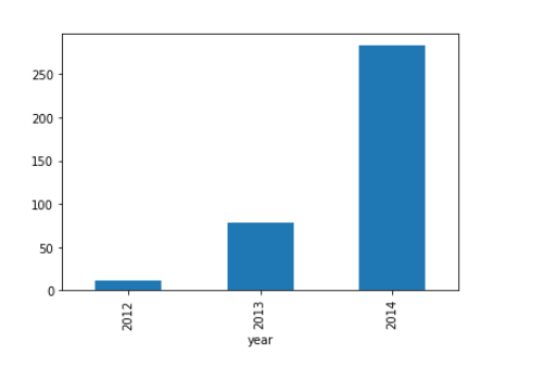
Our first hypothesis was traffic will increase as the years pass by. So let’s look at the yearly passenger count.

train.groupby('year')['Count'].mean().plot.bar()

We see an exponential growth in the traffic with respect to year which validates our hypothesis.

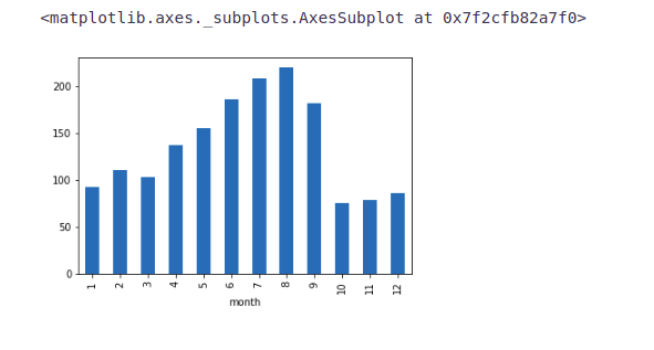
Our second hypothesis was about the increase in traffic from May to October. So, let’s see the relation between count and month.

train.groupby('month')['Count'].mean().plot.bar()

Here we see a decrease in the mean passenger count in the last three months. This does not look right. Let’s look at the monthly mean of each year separately.

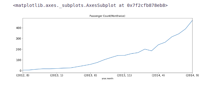
temp=train.groupby(['year', 'month'])['Count'].mean() 
temp.plot(figsize=(15,5), title= 'Passenger Count(Monthwise)', fontsize=14)

• We see that the months 10, 11, and 12 are not present for the year 2014 and the mean value for these months in the year 2012 is significantly less.
• Since there is an increasing trend in our time series, the mean value for the rest of the months will be more because of their larger passenger counts in the year 2014 and we will get a smaller value for these 3 months.
• In the above line plot, we can see an increasing trend in monthly passenger count and the growth is approximately exponential.

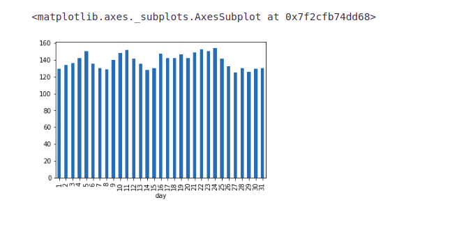
Let’s look at the daily mean of passenger count.

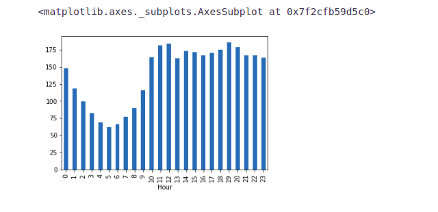
train.groupby('day')['Count'].mean().plot.bar()

We are not getting many insights from the day-wise count of the passengers.  We also made a hypothesis that the traffic will be more during peak hours. So let’s see the mean hourly passenger count.

train.groupby('Hour')['Count'].mean().plot.bar()

• It can be inferred that the peak traffic is at 7 PM and then we see a decreasing trend till 5 AM.
• After that, the passenger count starts increasing again and peaks again between 11 AM and 12 Noon.

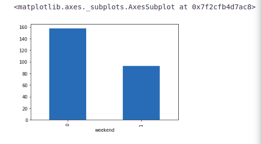
Let’s try to validate our hypothesis in which we assumed that the traffic will be more on weekdays.

train.groupby('weekend')['Count'].mean().plot.bar()

It can be inferred from the above plot that the traffic is more on weekdays as compared to weekends which validates our hypothesis.

Now we will try to look at the day-wise passenger count.

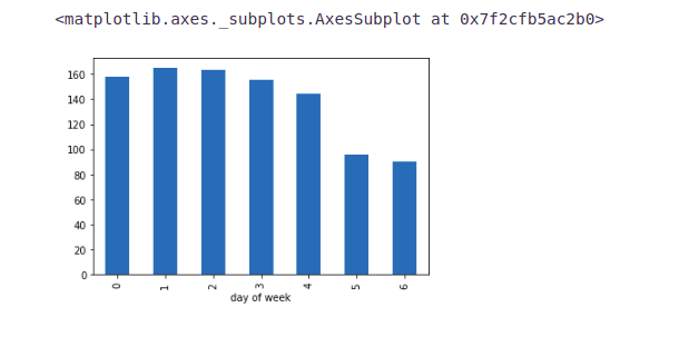
Note:-  0 is the starting of the week, i.e., 0 is Monday and 6 is Sunday.

train.groupby('day of week')['Count'].mean().plot.bar()

From the above bar plot, we can infer that the passenger count is less for Saturday and Sunday as compared to the other days of the week. Now we will look at basic modeling techniques. Before that, we will drop the ID variable as it has nothing to do with the passenger count.

train=train.drop(‘ID’,1)

As we have seen that there is a lot of noise in the hourly time series, we will aggregate the hourly time series into daily, weekly, and monthly time series to reduce the noise and make it more stable and hence would be easier for a model to learn.

train.Timestamp = pd.to_datetime(train.Datetime,format='%d-%m-%Y %H:%M') 
train.index = train.Timestamp 
hourly = train.resample('H').mean() 
daily = train.resample('D').mean() 
weekly = train.resample('W').mean() 
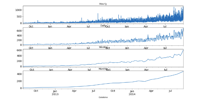
monthly = train.resample('M').mean()

Let’s look at the hourly, daily, weekly, and monthly time series.

fig, axs = plt.subplots(4,1) 
hourly.Count.plot(figsize=(15,8), title= 'Hourly', fontsize=14, ax=axs[0])
daily.Count.plot(figsize=(15,8), title= 'Daily', fontsize=14, ax=axs[1])
weekly.Count.plot(figsize=(15,8), title= 'Weekly', fontsize=14, ax=axs[2]) 
monthly.Count.plot(figsize=(15,8), title= 'Monthly', fontsize=14, ax=axs[3]) 
plt.show()

We can see that the time series is becoming more and more stable when we are aggregating it on a daily, weekly and monthly basis.

But it would be difficult to convert the monthly and weekly predictions to hourly predictions, as first we have to convert the monthly predictions to weekly, weekly to daily, and daily to hourly predictions, which will become a very expanded process. So, we will work on the daily time series.

test.Timestamp = pd.to_datetime(test.Datetime,format='%d-%m-%Y %H:%M') 
test.index = test.Timestamp 
test = test.resample('D').mean() 
train.Timestamp = pd.to_datetime(train.Datetime,format='%d-%m-%Y %H:%M')
 train.index = train.Timestamp  
train = train.resample('D').mean()

Modeling Techniques and Evaluation

As we have validated all our hypothesis, let’s go ahead and build models for Time Series Forecasting. But before we do that, we will need a dataset(validation) to check the performance and generalization ability of our model. Below are some of the properties of the dataset required for the purpose in this article for (Time Series Forecasting).

• The dataset should have the true values of the dependent variable against which the predictions can be checked. Therefore, the test dataset cannot be used for this purpose.
• The model should not be trained on the validation dataset. Hence, we cannot train the model on the training dataset and validate it as well.

So, for the above two reasons, we generally divide the train dataset into two parts. One part is used to train the model and the other part is used as the validation dataset. Now there are multiple ways to divide the training dataset such as Random Division etc.

Splitting the data into the training and validation part

Now we will divide our data into train and validation. We will make a model on the train part and predict on the validation part to check the accuracy of our predictions.

NOTE:-  It is always a good practice to create a validation set that can be used to assess our models locally. If the validation metric(rmse) is changing in proportion to the public leaderboard score, this would imply that we have chosen a stable validation technique.

To divide the data into training and validation sets, we will take the last 3 months as the validation data and the rest as training data. We will take only 3 months as the trend will be the most in them. If we take more than 3 months for the validation set, our training set will have fewer data points as the total duration is of 25 months. So, it will be a good choice to take 3 months for the validation set.

The starting date of the dataset is 25-08-2012 as we have seen in the exploration part and the end date is 25-09-2014.

Train=train.ix['2012-08-25':'2014-06-24'] valid=train.ix['2014-06-25':'2014-09-25']

• We have done time-based validation here by selecting the last 3 months for the validation data and the rest in the train data. If we would have done it randomly it may work well for the training dataset but will not work effectively on the validation dataset.
• Let’s understand it in this way: If we choose the split randomly it will take some values from the starting and some from the last years as well. It is similar to predicting the old values based on the future values which is not the case in a real scenario. So, this kind of split is used while working with time-related problems.

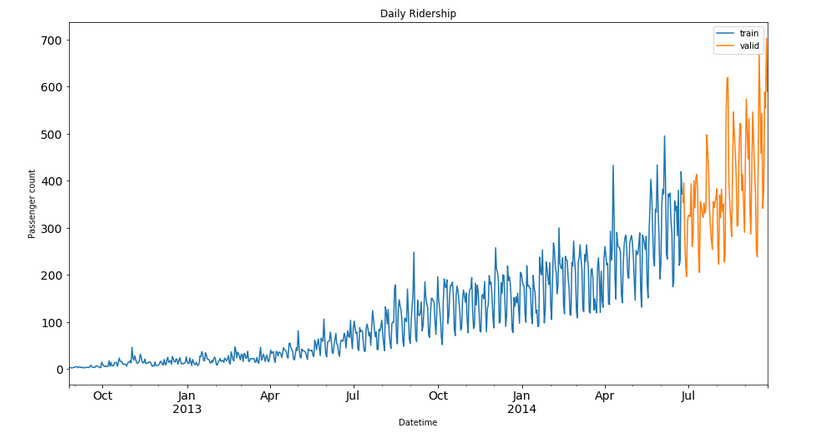
Now we will look at how the train and validation part has been divided.

Train.Count.plot(figsize=(15,8), title= 'Daily Ridership', fontsize=14, label='train') 
valid.Count.plot(figsize=(15,8), title= 'Daily Ridership', fontsize=14, label='valid') 
plt.xlabel("Datetime") plt.ylabel("Passenger count") 
plt.legend(loc='best') plt.show()

Here the blue part represents the train data and the orange part represents the validation data.

We will predict the traffic for the validation part and then visualize how accurate our predictions are. Finally, we will make predictions for the test dataset.

Time Series Forecasting Models

We will look at various models for Time Series Forecasting. Methods which we will be discussing for the forecasting are:

1. Naive Approach
2. Moving Average
3. Simple Exponential Smoothing
4. Holt’s Linear Trend Model

We will discuss each of these methods in detail now.

1) Naive Approach

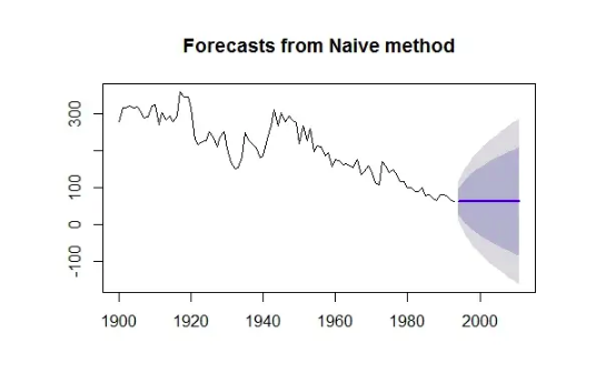
In this forecasting technique, we assume that the next expected point is equal to the last observed point. So we can expect a straight horizontal line as the prediction. Let’s understand it with an example and an image:

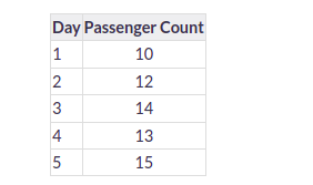
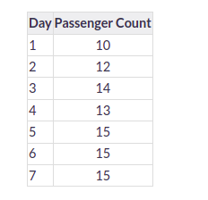
Suppose we have passenger count for 5 days as shown below:

And we have to predict the passenger count for the next 2 days. A naive approach will assign the 5th day’s passenger count to the 6th and 7th day, i.e., 15 will be assigned to the 6th and 7th day.

Now let’s understand it with an example:

Example:-

The blue line is the prediction here. All the predictions are equal to the last observed point.

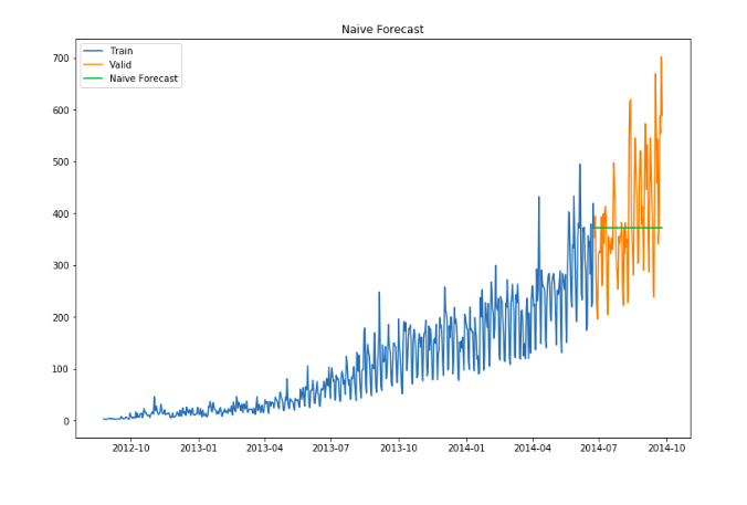
Let’s make predictions using the naive approach for the validation set.

dd= np.asarray(Train.Count) 
y_hat = valid.copy() 
y_hat['naive'] = dd[len(dd)-1] 
plt.figure(figsize=(12,8)) 
plt.plot(Train.index, Train['Count'], label='Train') 
plt.plot(valid.index,valid['Count'], label='Valid') 
plt.plot(y_hat.index,y_hat['naive'], label='Naive Forecast') 
plt.legend(loc='best') 
plt.title("Naive Forecast") 
plt.show()

• We can calculate how accurate our predictions are using rmse(Root Mean Square Error).
• rmse is the standard deviation of the residuals.
• Residuals are a measure of how far from the regression line data points are.
• The formula for rmse is:

                                        rmse=sqrt∑i=1N1N(p−a)2

We will now calculate RMSE to check the accuracy of our model on the validation data set.

from sklearn.metrics import mean_squared_error 
from math import sqrt 
rms = sqrt(mean_squared_error(valid.Count, y_hat.naive)) 
print(rms)

We can infer that this method is not suitable for datasets with high variability. We can reduce the rmse value by adopting different techniques.

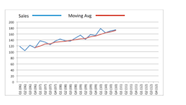
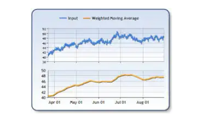
2) Moving Average

• In this technique, we will take the average of the passenger counts for the last few time periods only.

Let’s take an example to understand it:

Example

Here the predictions are made on the basis of the average of the last few points instead of taking all the previously known values.

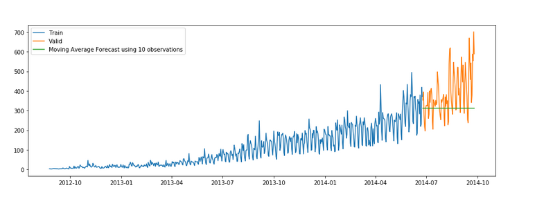
Let’s try the rolling mean for the last 10, 20, and 50 days and visualize the results.

y_hat_avg = valid.copy() 
y_hat_avg['moving_avg_forecast'] = Train['Count'].rolling(10).mean().iloc[-1] 
plt.figure(figsize=(15,5)) 
plt.plot(Train['Count'], label='Train') 
plt.plot(valid['Count'], label='Valid') 
plt.plot(y_hat_avg['moving_avg_forecast'], 
                label='Moving Average Forecast using 10 observations')

plt.legend(loc='best') 
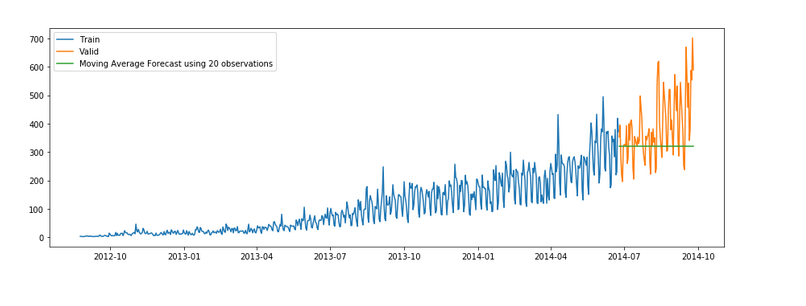
plt.show()

y_hat_avg = valid.copy() 
y_hat_avg['moving_avg_forecast'] = Train['Count'].rolling(20).mean().iloc[-1] 
plt.figure(figsize=(15,5)) 
plt.plot(Train['Count'], label='Train') 
plt.plot(valid['Count'], label='Valid') 
plt.plot(y_hat_avg['moving_avg_forecast'], 
                label='Moving Average Forecast using 20 observations') 
plt.legend(loc='best') 
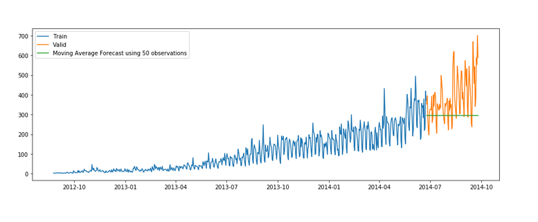
plt.show()

y_hat_avg = valid.copy() 
y_hat_avg['moving_avg_forecast'] = Train['Count'].rolling(50).mean().iloc[-1] 
plt.figure(figsize=(15,5)) 
plt.plot(Train['Count'], label='Train') 
plt.plot(valid['Count'], label='Valid') 
plt.plot(y_hat_avg['moving_avg_forecast'], 
                    label='Moving Average Forecast using 50 observations') 
plt.legend(loc='best') 
plt.show()

We took the average of the last 10, 20, and 50 observations and predicted based on that. This value can be changed in the above code in .rolling().mean() part. We can see that the predictions are getting weaker as we increase the number of observations.

rms = sqrt(mean_squared_error(valid.Count, y_hat_avg.moving_avg_forecast)) 
print(rms)

3) Simple Exponential Smoothing

In this technique, we assign larger weights to more recent observations than to observations from the distant past.

The weights decrease exponentially as observations come from further in the past, the smallest weights are associated with the oldest observations.

NOTE:- – If we give the entire weight to the last observed value only, this method will be similar to the naive approach. So, we can say that the naive approach is also a simple exponential smoothing technique where the entire weight is given to the last observed value.

Let’s look at an example of simple exponential smoothing:

Example

Here the predictions are made by assigning larger weight to the recent values and lesser weight to the old values.

from statsmodels.tsa.api 
import ExponentialSmoothing, SimpleExpSmoothing, Holt 
y_hat_avg = valid.copy() 
fit2 = SimpleExpSmoothing(np.asarray(Train['Count'])).fit(smoothing_level=0.6,
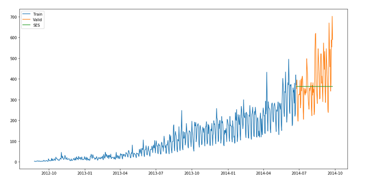
        optimized=False) y_hat_avg['SES'] = fit2.forecast(len(valid))

plt.figure(figsize=(16,8))  
plt.plot(Train['Count'], label='Train') 
plt.plot(valid['Count'], label='Valid') 
plt.plot(y_hat_avg['SES'], label='SES') 
plt.legend(loc='best') 
plt.show()

rms = sqrt(mean_squared_error(valid.Count, y_hat_avg.SES)) 
print(rms)

113.43708111884514

We can infer that the fit of the model has improved as the rmse value has reduced.

4) Holt’s Linear Trend Model

• It is an extension of simple exponential smoothing to allow forecasting of data with a trend.
• This method takes into account the trend of the dataset. The forecast function in this method is a function of level and trend.

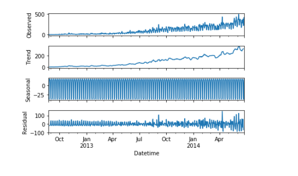
First of all let us visualize the trend, seasonality, and error in the series.

We can decompose the time series into four parts.

• Observed, which is the original time series.
• Trend, which shows the trend in the time series, i.e., increasing or decreasing behavior of the time series.
• Seasonal, which tells us about the seasonality in the time series.
• Residual, which is obtained by removing any trend or seasonality in the time series.

Let’s visualize all these parts.

import statsmodels.api as sm 
sm.tsa.seasonal_decompose(Train.Count).plot() 
result = sm.tsa.stattools.adfuller(train.Count) 
plt.show()

An increasing trend can be seen in the dataset, so now we will make a model based on the trend.

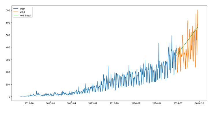
y_hat_avg = valid.copy() 
fit1 = Holt(np.asarray(Train['Count'])).fit(smoothing_level = 0.3,
        smoothing_slope = 0.1) y_hat_avg['Holt_linear'] = fit1.forecast(len(valid)) 
plt.figure(figsize=(16,8))

plt.plot(Train['Count'], label='Train')
plt.plot(valid['Count'], label='Valid') 
plt.plot(y_hat_avg['Holt_linear'], label='Holt_linear') 
plt.legend(loc='best') 
plt.show()

We can see an inclined line here as the model has taken into consideration the trend of the time series.

Let’s calculate the rmse of the model.

rms = sqrt(mean_squared_error(valid.Count, y_hat_avg.Holt_linear)) 
print(rms)

112.94278345314041

It can be inferred that the rmse value has decreased.

Now we will be predicting the passenger count for the test dataset using various models.

Conclusion on Time Series Forecasting

In this article on Time Series Forecasting, we solved the problem of time series in the daily data. We are trying to make a weekly time series, make predictions for that series, and then
distribute those predictions into daily and then hourly predictions. We can use a combination of models(ensemble) to reduce the rmse. To read more about ensemble techniques.

We learned about Time Series Forecasting data and how to build forecasting models using time series data using an example problem. We also learned about various components of time series data and how it differs from Regression data. I hope the articles helped you understand how to deal with time-series data, and how to find daily basis records from time series, we are going to use this technique, and apply it in a few domains such as the sales prediction analysis domain.

The media shown in this article is not owned by Analytics Vidhya and is used at the Author’s discretion.

Kajal Kumari 19 May 2023