Introduction
Today everything in this world has become faster and more automated. Be it the suggestions we get for buying groceries or writing an email at the last minute. You name it, and there are several options for you to choose from. Here’s the thing: no human is sitting on the other side and suggesting all these. It’s all the machine learning lifecycle doing it for you. For example, Grammarly is helping me to write this article correctly! 🙂
What is Machine Learning Lifecycle?
So, what is Machine Learning Lifecycle? The answer is in the term itself! So, we know that the term machine learning refers to the computer’s ability to learn by itself without giving it instructions. And now another term, lifecycle.
So, we can say the machine learning lifecycle is a recurrent or a cyclical process that is followed by data science projects to find a solution to the problem or project, analyze and draw inferences from patterns in data, bring out better insights, help in better decision making, finally helping the business to have good growth. Why is it a cycle? So, whenever the science is applied to the data with newer modifications, it gives a better result.
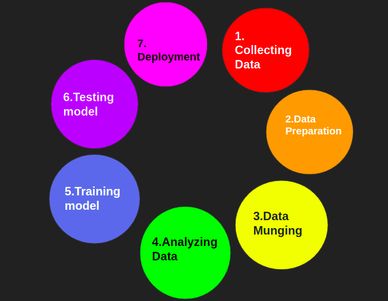
Steps involved in Machine Learning Lifecycle
- Collection/gathering of the data: This is the first step of the machine learning life cycle. The data can be from various sources, from banks, hospitals, surveys, queries, reports, social media, OTT platform data, and many more. They would be in large amounts because they form every minute, every second.
- Data preparation: This is the second step of the machine learning life cycle. Let’s take an example to understand this. So, it’s the weekend, and we wish to clean the study room, which has been pending for many days and has become very untidy. Now understanding where to keep things in an organized way needs some planning or reshaping.
So, the colored pencils and marker pens cannot be placed in the bookrack. Also, the other way round, the books cannot be put on the pen stand. So, here we are, making changes that would help us in further data analysis. The data comes from a large variety of sources, but to make it into an understandable form such that the people who analyze the data or the data scientists may understand it, is what is performed in this step.
Often the data preparation and the data munging/cleaning/wrangling step seem to be a lot similar. But here’s the catch, the former is performed before the iterative/repetitive analysis, i.e., it’s only performed for the first time, and the latter is performed during the iterative analysis.
- Data Munging: This is the third step in the machine learning life cycle and refers to the cleaning of the data, hence also called the data cleaning or the data wrangling step, where the raw data is converted into a much more useable form, structuring the data in such a way such that it can be easier to perform analysis in the further steps.
Here, the quality information is sieved out that would help in the process of decision making. Also, the more the cleaned data is, the more the chances will be that our model, which we would build, later on, would have higher accuracy. It can include several things, including removing outliers from the data/dataset, handling/removing missing values, converting the necessary data types, and many more.
- Analyzing the data: Now as we have the cleaned data, we are ready for the next step, where we develop models and test using analytical methods. In this step, we will model and visualize our data to extract major and helpful information with the help of several machine learning tools and techniques and analyze its outcome.
Let’s say we have now kept everything in its proper place in our study room, but something needs to be fixed. I have colored pencils from different brands, ranging from expensive to cheaper ones. Surprisingly the cheaper brands work fine instead than the costlier brands. So, this is something I will keep in my mind when I go and buy these pencils.
- Training the model: In this step, we train the model. Broadly saying, it’s the process where machine learning algorithms are fed with ample training data to learn from to better their performance for a better outcome of the problem.
We need a lot of clean, processed data to perform this efficiently. We need a lot of data so the machine can learn much, and the predictions will be much better. For the first time, let’s say you are shown just ten pictures of cats and dogs. Not necessary that those ten pictures might be enough for you to learn, and why is that so? You would get its answer in the next part, i.e., in the test.
- Testing the model: Now that our model has been tested on an ample number of datasets, it’s ready for the testing part. Here’s the answer to the question we had in the last paragraph.
Now, let’s say that after training with only those ten pictures, you are shown an image of the Chow Chow breed or the Hmong breed to test or check how much you(here, the machine) have learned. You won’t be able to answer because you learned from fewer data, and it didn’t contain these breeds’ pictures. Had it been a large amount of data, higher chances would have been that it would have covered the pictures of the rare breeds, too, including the above ones.
- Deployment: Here, the built model is put into a working, live environment so that it can be used according to the business needs/requirements. They are done so that the model is linked with the apps through APIs, so users can use it efficiently and fulfill their purpose.
Case Study
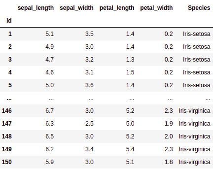
So, to understand all the steps of the machine learning life cycle in a much finer way, we’ll be understanding it with the help of a dataset. Here we’ll be using the Iris dataset. You can easily get it from here. Let’s have a brief understanding of this dataset. So, this dataset is about the details of a flowery plant with its subfamily named Iris. The dataset has three variants/species of this subfamily: Setosa, Versicolor, and Virginica.
This particular dataset has 4 numerical features and 1 tri-class target variable. So the 4 numerical features are input variables(sepal_length, sepal_width, petal_length and petal_width). Let’s say we are scientists and need to identify the species of the flower based on the above-mentioned features. This is what the machine is gonna learn and then perform. So, let’s get started!
1. Getting the Data: Our first step is to get the data. This is already a structured dataset you can get from anywhere. Now, that we have the data with us, we can go to the next step.
2. Data Preparation: Let’s come to the next step, i.e., the Data Preparation step. Over here, in this, we’ll try to check if the data meets the analyzing standards or do we need to make some changes to make it analyzable? and all that.
Let’s start by importing the libraries.
import numpy as np
import pandas as pd
import matplotlib.pyplot as plt
import seaborn as sns
import warnings
warnings.filterwarnings('ignore')
Now, we’ll have a good look at the data to understand it better.
#import numpy as np
import pandas as pd
#import matplotlib.pyplot as plt
#import seaborn as sns
import warnings
warnings.filterwarnings('ignore')
# loading and reading through the dataset
iris_df = pd.read_csv('Iris.csv')
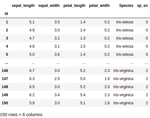
# first few rows of the dataset
print(iris_df.head())
# last few rows of the dataset
print(iris_df.tail())
What we can see from the above output is that it needs a little formatting to make it easier for analysis. We can perform the following change:
# changing a column to index
iris_df = iris_df.set_index('Id')
.png)
We can see that the column names are not that easy to read, so we change the column names too to make them easier to analyze.
iris = iris_df.rename(columns={'SepalLengthCm':'sepal_length',
               'SepalWidthCm':'sepal_width',
               'PetalLengthCm':'petal_length',
               'PetalWidthCm':'petal_width'})
So now, we are ready for the next step, i.e., Data Munging/Data Cleaning/Data Wrangling. In this step, we’ll be cleaning the data in a way, to make it more presentable, and make it easier for analysis. We’ll start by looking for missing values.
# checking, if the dataset has some null values
iris.isnull().sum()
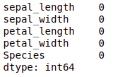
So, we can see no missing value in our dataset. Had there been such missing value, we would have needed to impute it with something else. But as we don’t have any such as of now, it saves the time for imputation.
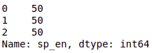
Suppose we wish to know how many data points for each species are present.
# How many flowers does each species have?
iris_df['Species'].value_counts()
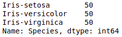
We can see from the above output that the data with which we are working is balanced(almost equal no. of data points for each column/class). Then what is an unbalanced dataset? The answer is that if there is a huge difference between the no. of data points from each column/class, it’s unbalanced.
Let’s see with an example: Say we have patients’ data and label them as diabetic or non-diabetic based on some input parameters: the medical tests performed on the people. We found a maximum number of people are non-diabetic, and very few are diabetic. This huge difference can be termed an imbalance.
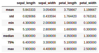
Let’s see the five-number summary of our data to see how our data is distributed.
irfi = iris.describe()
irfi = irfi.drop('count')
irfi = irfi.rename({'50%' : 'median'}) # we are renaming the row from 50% to median to  have a better understanding
irfi
Let’s go with the visualization. Let’s first try to know which one variable among the four variables can be more suitable to distinguish between the species, and here’s where the univariate analysis comes into the picture.
We’ll try to build a plot where we’ll try to distinguish between all three species using all variables individually.
sns.FacetGrid(iris, hue='Species', size=4).map(sns.histplot, 'petal_length', bins=15).add_legend()
plt.show()
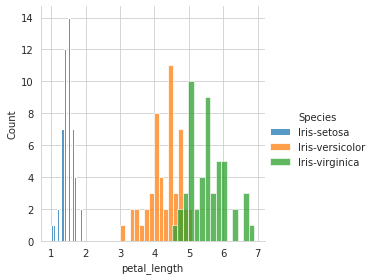
From the above plot, we can see that the setosa can be distinguished from the other two species, that is, Versicolor and Virginica (these two have overlapping).
We analyzed this using one variable -> petal_length
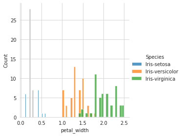
# using petal_width
sns.FacetGrid(iris, hue='Species', size=4).map(sns.histplot, 'petal_width', bins=20).add_legend()
plt.show()
# using petal_width
sns.FacetGrid(iris, hue='Species', size=4).map(sns.histplot, 'petal_width', bins=20).add_legend()
plt.show()
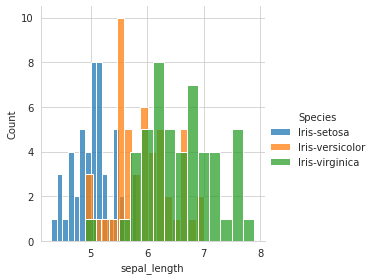
# using sepal_length
sns.FacetGrid(iris, hue='Species', size=4).map(sns.histplot, 'sepal_length', bins=15).add_legend()
plt.show()
# using sepal_width
sns.FacetGrid(iris, hue='Species', size=4).map(sns.histplot, 'sepal_width', bins=25).add_legend()
plt.show()
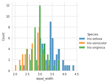
Out of the four variables, when plotted individually, sepal_length and sepal_width is the worst feature to distinguish between the species.
petal_length and petal_width are the better features to distinguish(although there’s some overlap Versicolor and virginica)
petal_length being the best feature, followed by petal_width, followed by sepal_length, and lastly sepal_width.
Let’s go with the Bivariate Analysis. We’ll use the scatter plot to see how the data points are spread and how much they are scattered.
sns.set_style('whitegrid') # form grid pattern when showing the graph
sns.FacetGrid(iris, hue='Species', # hue tells by which parameter/column should i colour my points
              size=4).map(plt.scatter, 'sepal_length', 'sepal_width').add_legend()
plt.show()
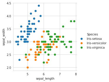
Okay, Awesome! Now we have a better visualization. What do we infer?
1. Setosa is distinguishable from the Versicolor and Virginica -> linearly separable if we draw a line in such a way that on one side of the line, we have only the setosa,
2. And on the other side, we have Versicolor+Virginica overlapped on one another, differentiating between two species, i.e., Versicolor and virginica is harder(as they overlap).
We have four feature datasets (sepal_length, sepal_width, petal_length, petal_width), and we can’t use a scatter plot to view the four-dimensional data, so here we can use a Pair Plot. Here using 4 parameters, two getting paired each time, we can 6 such unique combinations and a total of 16 combinations(repeated ones+unique).
sns.set_style('whitegrid')
sns.pairplot(iris, hue='Species', size=2)
plt.show()
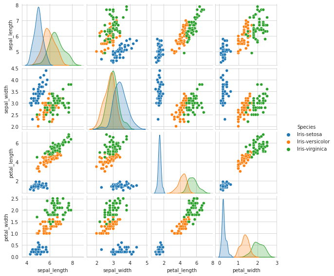
What do we infer from the above plot? (We’re focusing on the top 6 scatter plots from the diagonal)
- Petal Length, Petal Width -> The petal length and width feature is a better distinguisher(distinguishing feature) between the species than other parameters/features.
- Look at the plot (3,4) 3rd row, 4th column. All the species are somewhat well separated based on petal_width and petal_length.2.1 If we are asked to predict the species type based on petal_width and petal_length, we can say that: if petal_width >= 1 and <=2, along with if the petal_width 2.5, then its Versicolor(minute overlapping)
Let’s say we want to plot the correlation between the variables.
iris.corr()
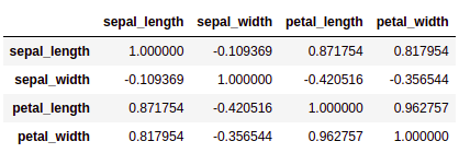
Let’s try to understand the above output in a graphical manner
corr = iris.corr()
fig, ax = plt.subplots(figsize = (4,4))
sns.heatmap(corr, annot=True, ax=ax, cmap='PiYG')
plt.show()
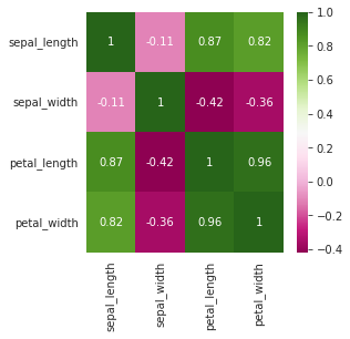
A high correlation can be seen between petal_width and petal_length. We could have neglected one out of the two variables that have a high correlation, but here we aren’t doing that because we only have 4 variables.
Let’s go to the next step: building the model, training it, and testing it. We’ll start by label encoding. Here, in this particular dataset, we have multiple categories in one of the columns(in the form of words: Output variable -> Species). Through this process, we’ll convert these labels into a numeric form such that the machine understands it.
from sklearn.preprocessing import LabelEncoder
lbe = LabelEncoder()
iris['sp_en'] = lbe.fit_transform(iris['Species'])  # using the fit_transform to transform the the categories in the Species column to numeric form, keeping it in another new column named sp_en
iris
iris['sp_en'].value_counts()
Now, we’ll train the model.
We are splitting our data to train 80% of the data and test 20% of the data.
from sklearn.model_selection import train_test_split
X = iris.drop(columns=['Species','sp_en'])
Y = iris['sp_en']
x_train, x_test, y_train, y_test = train_test_split(X, Y, test_size=0.2)
Logistic Regression
from sklearn.linear_model import LogisticRegression
# initialize the model
model = LogisticRegression()
# training the model
model.fit(x_train, y_train)
# checking the performance
a = model.score(x_test, y_test) # testing the model with test dataset
acc=a*100
acc="{:.3f}".format(acc)
#print('Accuracy: ', a*100,'%')
print('Accuracy is: '+acc+str('%'))

Let’s check the accuracy with another model
KNN
from sklearn.neighbors import KNeighborsClassifier
model1 = KNeighborsClassifier()
model1.fit(x_train, y_train)
# checking the performance
a = model1.score(x_test, y_test) # testing the model with test dataset
acc=a*100
acc="{:.3f}".format(acc)
#print('Accuracy: ', a*100,'%')
print('Accuracy is: '+acc+str('%'))

So, the accuracy which we got is quite good. Using some more models and hyperparameter tuning, we might get better accuracy.
Conclusion
So, in this article, we learned about what exactly a machine learning lifecycle is. How does it perform, its components, and how does it help make better decision-making? We also saw a practical example that showed us how all the steps are being performed from first to last. Here, we understood the lifecycle of machine learning using the iris dataset.


