Doing Data Exploration the right way – GRE Scores Case Study

This article was published as a part of the Data Science Blogathon

Meaningful data exploration is very important. There are often, no definite guides or roadmaps to execute data exploration. Every data science professional or student has at some point, has arrived at a point, we’re looking at raw data, they don’t know how to proceed. So, putting it all together, data exploration is the process of uncovering various hidden aspects of the data at hand.

Importance of Data Exploration:

Data exploration helps in making better decisions with the data. Often, certain types of ML/DL algorithms are more suitable for certain types of data. With a good idea of the data distribution, we can ask better questions about the data.

The dataset consists of various data fields which are important while applying to college.

Data:

1. GRE Scores ( out of 340 )
2. TOEFL Scores ( out of 120 )
3. University Rating ( out of 5 )
4. Statement of Purpose and Letter of Recommendation Strength ( out of 5 )
5. Undergraduate GPA ( out of 10 )
6. Research Experience ( either 0 or 1 )
7. Chance of Admit ( ranging from 0 to 1 )

We will have a look at how much GRE scores can determine your chance of admission.

Are GRE scores important?

We will be having a look at how important GRE scores are for admissions and how much they matter. We shall try to understand the relation between the GRE score and other variables and try to see how they affect the admission chance.

I will leave a link to the code at the end of the article.

import numpy as np 
import pandas as pd

import matplotlib.pyplot as plt 
import seaborn as sns
%matplotlib inline

#reading the data
df= pd.read_csv("/kaggle/input/graduate-admissions/Admission_Predict.csv")

#how the data looks
df.head()

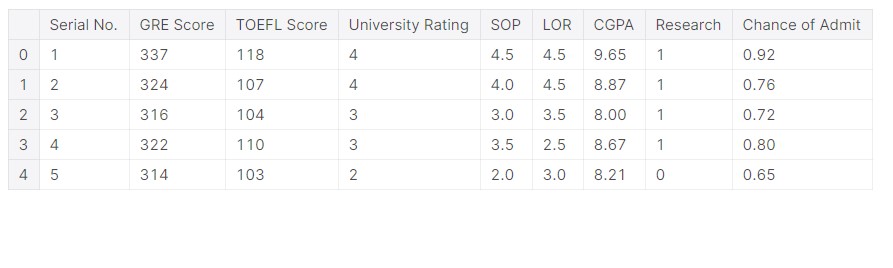
We can now have a look at the data, it looks like GRE scores are in the range of 300. It makes sense, as GRE has a full mark of 340. An important aspect of data exploration is that we need to relate it to real-life situations.

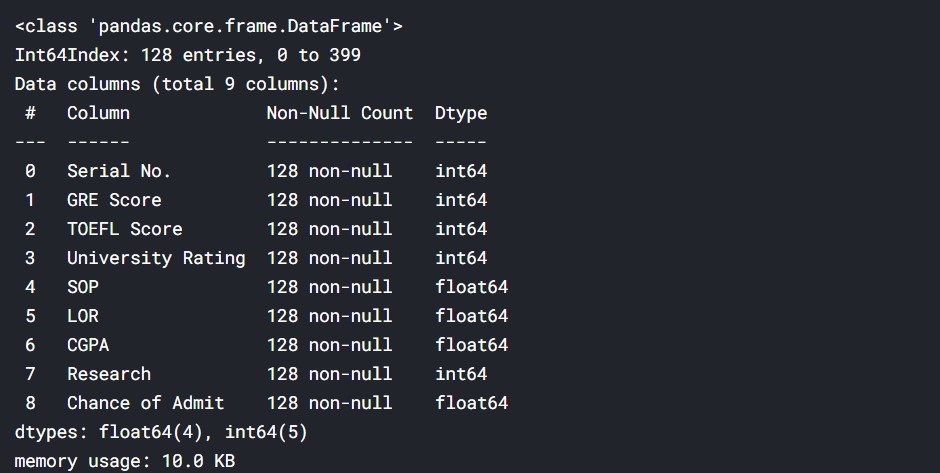
print("DATA INFORMATION AND DATA TYPES")
df.info()

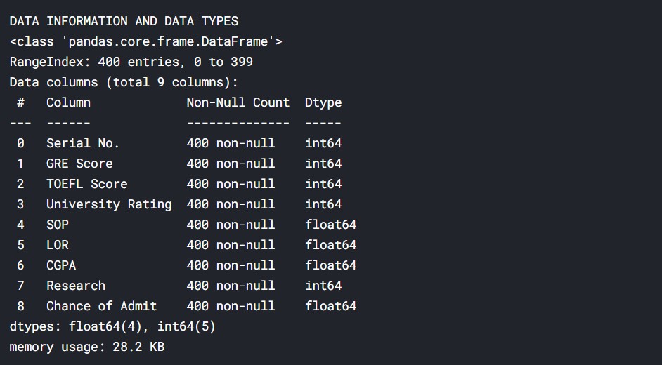
Basically, we get an idea about all the data types and how many data points we have, here 400.

print('MISSING DATA (IF ANY)')
df.isnull().sum()

So, none of the data fields is empty, which means we do not have to deal with missing values.

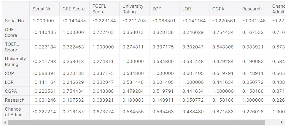
df.corr()

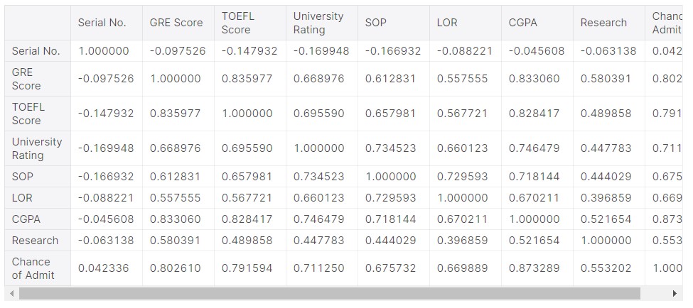
There is a 0.802 correlation between the GRE score and the chance of admission. So there might be a big chance that these variables (data) are highly related. In fact, the correlation is the second-highest, after the CGPA. So, we can determine that CGPA and GRE scores are most important in determining the chances of admission.

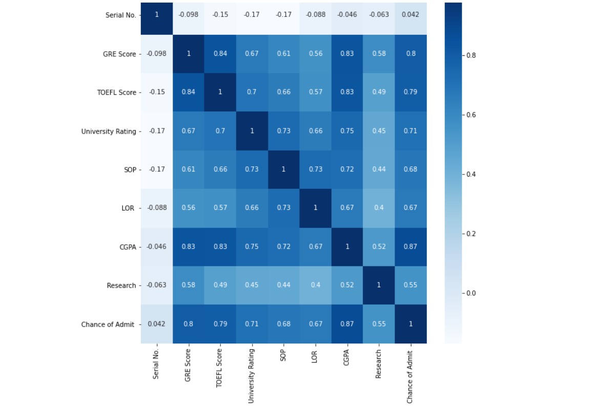
plt.figure(figsize = (10,10))
sns.heatmap(df.corr(),annot=True, cmap='Blues')

plt.subplots(figsize=(12,8))
plt.scatter(df["Chance of Admit "],df["GRE Score"])
plt.xlabel("Chance of Admit")
plt.ylabel("GRE Score")

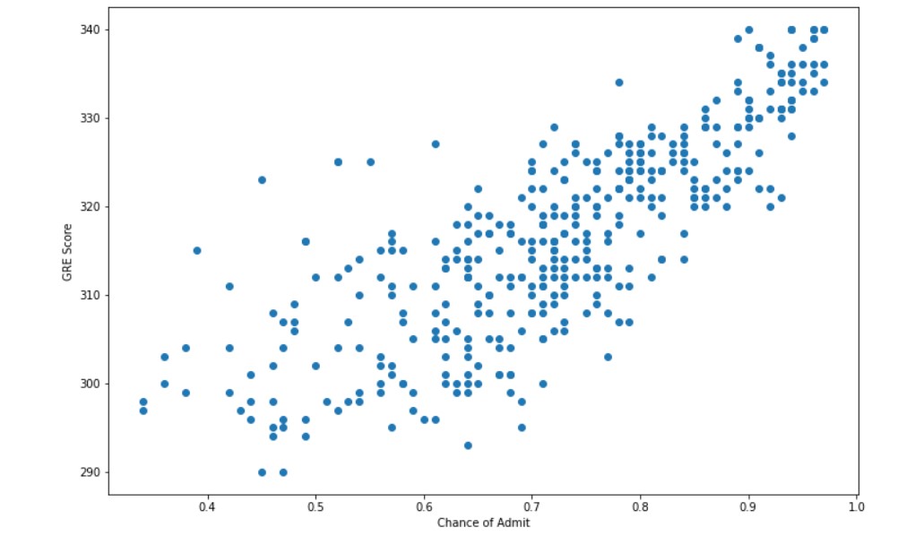
There does appear to be a connection between the two variables. Some exploration needs to be done.

plt.subplots(figsize=(12,8))
sns.regplot(x="GRE Score", y="Chance of Admit ", data=df)

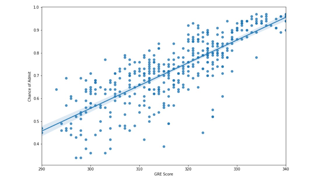
We are able to comfortably plot a linear regression line through the data. Let us try some other plots and take in other data, to understand the whole picture as a whole.

sns.jointplot(df["GRE Score"], df["Chance of Admit "], kind="kde", height=8, space=0)
plt.plot(figsize=(12,8))

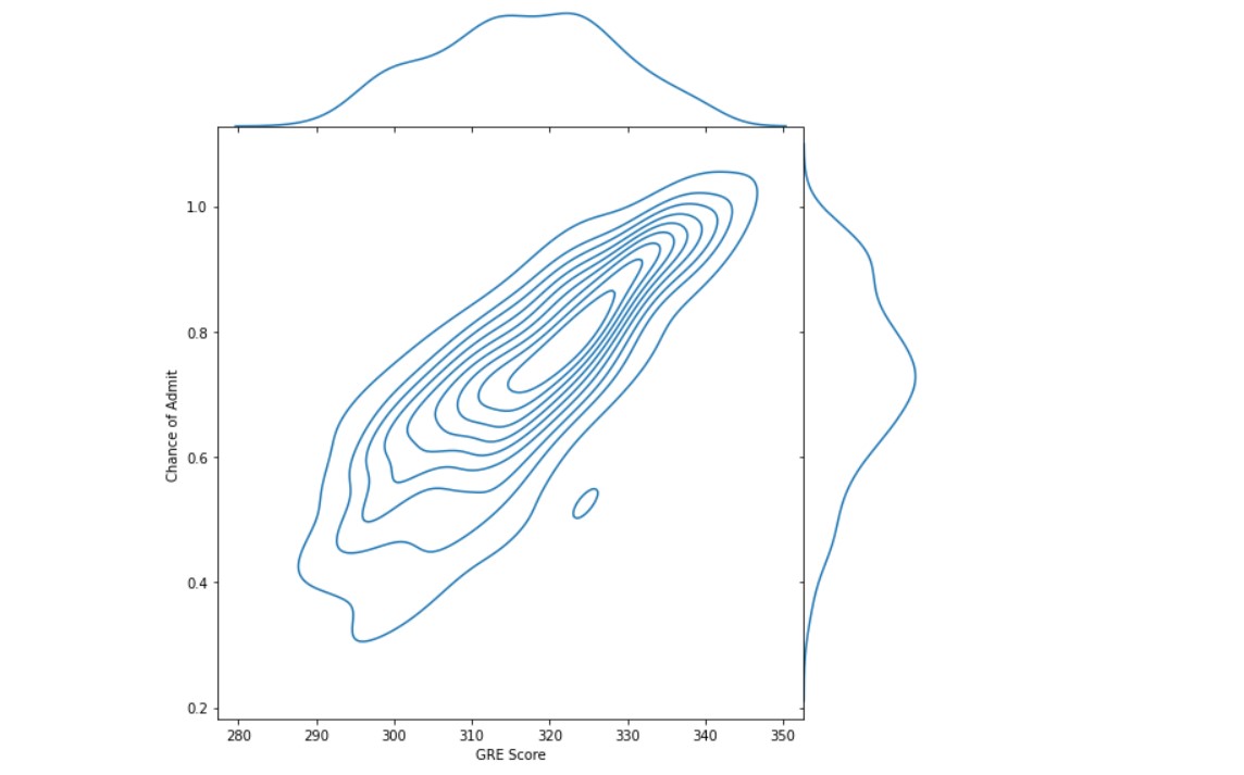
Let us see if the research experience of a candidate helps in getting admits.

sns.lmplot(x="GRE Score", y="Chance of Admit ", data=df, hue="Research",height= 8)

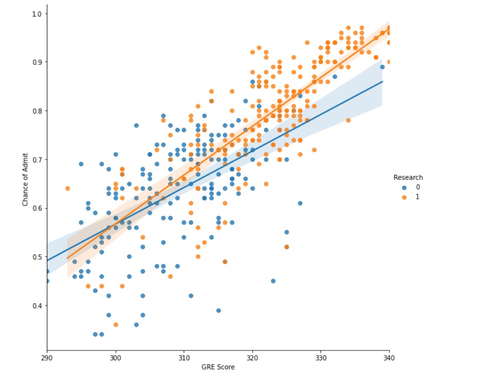
The data does show that candidates having research experience (orange in the figure), usually have more chance of admits. That being said, these candidates also have good GRE scores. So good GRE scores do indicate a good candidate profile.

Conclusion: Having research experience is very important.

Now, let us have a look at university ratings.

sns.lmplot(x="GRE Score", y="Chance of Admit ", data=df, hue="University Rating",height=8)

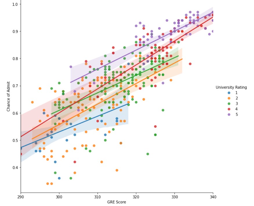
Observations :

• Students having higher GRE scores (>320) usually have a high chance of admission into the university with higher ratings (4/5).
• A lower GRE score has a lower chance of admission, that too for universities of low ratings.
• Students having a higher chance of admission, all have good GRE scores and University ratings of 4 or 5.

Now we take some data where we take chances of admit to being 0.8 or higher and check how important are GRE scores.

admit_high_chance= df[df["Chance of Admit "]>=0.8]

admit_high_chance.info()

#128 data taken

admit_high_chance.corr()

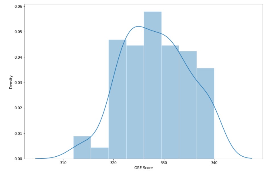
Now let us look at the distribution of Chance of Admit and GRE score.

plt.subplots(figsize=(12,8))
sns.set_theme(style="darkgrid")
sns.distplot( admit_high_chance["GRE Score"])

plt.subplots(figsize=(12,8))
sns.set_theme(style="darkgrid")
sns.distplot( admit_high_chance["Chance of Admit "])

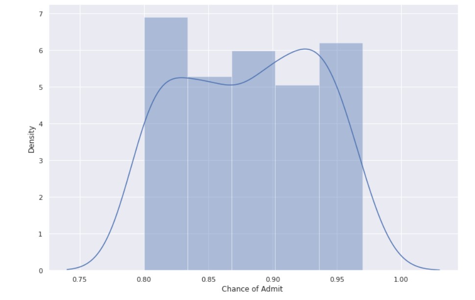
Observations :

1. For a higher chance of admission, the GRE score is also high.
2. Maximum GRE scores are in the range of 320-340.

Linear Regression between GRE Scores and the chance of admit:

X= df["GRE Score"].values

#bringing GRE score in a range of 0-1

X=X/340

y= df["Chance of Admit "].values

#sk learn train test split data

from sklearn.model_selection import train_test_split
X_train, X_test, y_train, y_test = train_test_split(X, y, test_size = 0.25)

#sk learn linear regression

from sklearn.linear_model import LinearRegression
lr = LinearRegression()

#training the model on training data
lr.fit(X_train.reshape(-1,1), y_train)

y_pred = lr.predict(X_test.reshape(-1,1))

#model score

lr.score(X_test.reshape(-1,1),y_test.reshape(-1,1))

Output: 0.6889753669343462

plt.subplots(figsize=(12,8))
plt.scatter(X_train, y_train, color = "red")
plt.plot(X_train, lr.predict(X_train.reshape(-1,1)), color = "green")
plt.title("GRE Score vs Chance of Admit")
plt.xlabel("GRE Score")
plt.ylabel("Chance Of Admit")
plt.show()

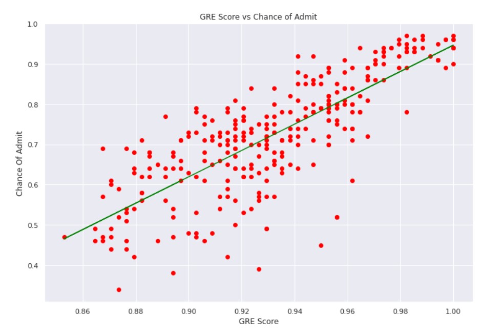
The model is not performing that well, but we do understand that there is a correlation between GRE scores and the chance of admit.

Let us try with a test input.

#test input

test= 320
val= test/340

val_out=lr.predict(np.array([[val]]))

print("Chance of admission :", val_out[0])

Chance of admission: 0.7540416752698649

Creating a Model on the entire data:

x = df.drop(['Chance of Admit ','Serial No.'],axis=1)
y = df['Chance of Admit ']

X_train, X_test, y_train, y_test = train_test_split(x,y,test_size=0.25, random_state = 7)

#random forest regression

from sklearn.ensemble import RandomForestRegressor

regr = RandomForestRegressor(max_depth=2, random_state=0, n_estimators=5)

regr.fit(X_train,y_train)

regr.score(X_test, y_test)

val=regr.predict([[325, 100, 3, 4.1, 3.7, 7.67, 1]])

print("Your chances are (in %):")
print(val[0]*100)

Output:

Your chances are (in %):

54.47694678499888

Conclusion:

1. GRE Score is important for admission.
2. Students having good GRE score, seem to have good overall profiles.
3. There are obviously exceptions, which comprise the outliers.

Final Words:

Data exploration can help in understanding the relevance of the data available to us and is a great way to start the whole Data Science process. Properly executed data exploration helps in get actionable insights from the data.

Code Link on Kaggle

About me:

Prateek Majumder

Data Science and Analytics | Digital Marketing Specialist | SEO | Content Creation

Connect with me on Linkedin.

Thank You.

The media shown in this article are not owned by Analytics Vidhya and are used at the Author’s discretion.

Prateek Majumder

Prateek is a dynamic professional with a strong foundation in Artificial Intelligence and Data Science, currently pursuing his PGP at Jio Institute. He holds a Bachelor's degree in Electrical Engineering and has hands-on experience as a System Engineer at TCS Digital, where he excelled in API management and data integration. Prateek also has a background in product marketing and analytics from his time with start-ups like AppleX and Milkie Way, Inc., where he was involved in growth campaigns and technical blog management. Recognized for his structured thinking and problem-solving abilities, he has received accolades like the Dr. Sudarshan Chakraborty Award for Best Student Performance. Fluent in multiple languages and passionate about technology, Prateek continues to expand his expertise in the rapidly evolving AI and tech landscape.