This article was published as a part of the Data Science Blogathon.
Overview
In this article, we will be predicting the profit from the startup’s dataset with the features available to us. We’re using the 50-startups dataset for this problem statement and we will be using the concept of Multiple linear regression to predict the profit of startups companies.
How do startups work?
Well, we can say that startups pipeline operates on the same principles which are similar to other MNCs the major difference between both of them is that on the one hand startups work to make products that are beneficial for the customers on a small scale while other established companies do that work on a large scale by re-doing something which is already being done.
How startups are being funded?
How startups are being funded?
As I mentioned above the startups are not such economical balanced company that has covered a path from an idea to a product so for the same reason no established investor will be going to come forward for those companies which don’t really have their market value hence, startups allow the early investors to start supporting in the format of seed funding which would help them to make a product out of their idea. In a nutshell, we can see that it’s hard to manage and analyze the investments and to make a profit out of them.
We need a way by which we can analyze our expenditure on the startups and then know a profit put of them!
How this model can help here?
This machine learning model will be quite helpful in such a situation where we need to find a profit based on how much we are spending in the market and for the market. In a nutshell, this machine learning model will help to find out the profit based on the amount which we spend from the 50 startups dataset.
About the 50 startups dataset
This particular dataset holds data from 50 startups in New York, California, and Florida. The features in this dataset are R&D spending, Administration Spending, Marketing Spending, and location features, while the target variable is: Profit. –Source.
- 1. R&D spending: The amount which startups are spending on Research and development.
- 2. Administration spending: The amount which startups are spending on the Admin panel.
- 3. Marketing spending: The amount which startups are spending on marketing strategies.
- 4. State: To which state that particular startup belongs.
- 5. Profit: How much profit that particular startup is making.
Table of content
- 1. Difference between Linear Regression and Multiple linear regression
- 2. Importing libraries
- 3. Analyzing the data
- 4. EDA on the dataset
- 1. Data Visualization
- 2. Feature exploration
- 5. Model development
- 6. Model evaluation
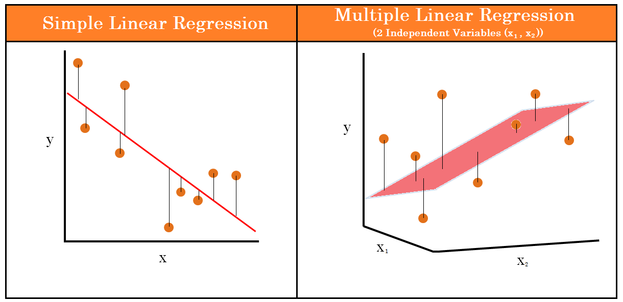
Difference between Linear regression and Multiple linear regression
The major difference between linear regression and multiple linear regression is that in linear regression there is only one independent variable while when we check out, Multiple linear regression there is more than one independent variable.
Let’s take an example of both the scenarios
- 1. Linear regression: When we want to predict the height of one particular person just from the weight of that person.
- 2. Multiple Linear regression: If we alter the above problem statement just a little bit like, if we have the features like height, age, and gender of the person and we have to predict the weight of the person then we have to use the concept of multiple linear regression.
Importing libraries & dataset
Python Code:
import numpy as np
import pandas as pd
# import seaborn as sns
# import matplotlib.pyplot as plt
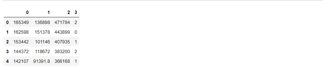
dataset = pd.read_csv('50_Startups.csv')
print(dataset.head())
Numerical/Statistical analysis of the dataset
dataset.describe()
Output:
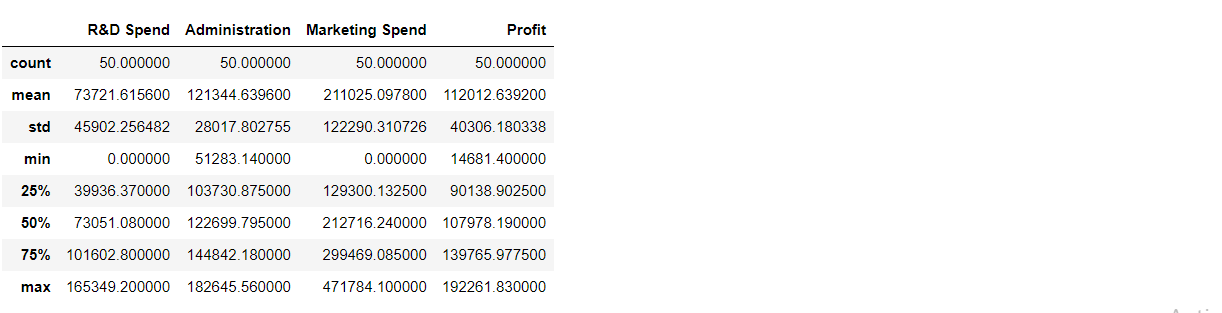
Dimensions of dataset
print('There are ',dataset.shape[0],'rows and ',dataset.shape[1],'columns in the dataset.')
Output:
There are 50 rows and 5 columns in the dataset.
Here we are trying to check if there are repeated values in the dataset or not.
print('There are',dataset.duplicated().sum(),'duplicate values in the dateset.') #using duplicated() pre-defined function
Output:
There are no repeating values in the dataset.
Check for NULL values
dataset.isnull().sum()
Output:
R&D Spend          0
Administration     0
Marketing Spend    0
State              0
Profit             0
dtype: int64
Inference: There are no null values in the dataset.
Schema of dataset
dataset.info()
Output:
RangeIndex: 50 entries, 0 to 49
Data columns (total 5 columns):
 #   Column           Non-Null Count  Dtype
---  ------           --------------  -----
 0   R&D Spend        50 non-null     float64
 1   Administration   50 non-null     float64
 2   Marketing Spend  50 non-null     float64
 3   State            50 non-null     object
 4   Profit           50 non-null     float64
dtypes: float64(4), object(1)
memory usage: 2.1+ KB
From the corr function, we can find the correlation between the columns.
c = dataset.corr()
c
Output:
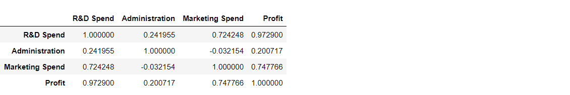
Inference: We can see that all three columns have a direct relationship with the profit, which is our target variable.
EDA on dataset
Correlation matrix
sns.heatmap(c,annot=True,cmap='Blues')
plt.show()
Output:
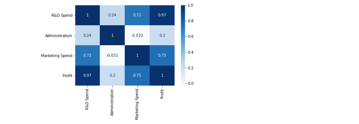
Inference: Here we can see the direct correlation with profit from how it is shown in the heatmap of the correlation plot.
Outliers detection in the target variable
outliers = ['Profit']
plt.rcParams['figure.figsize'] = [8,8]
sns.boxplot(data=dataset[outliers], orient="v", palette="Set2" , width=0.7) # orient = "v" : vertical boxplot ,
                                                                            # orient = "h" : hotrizontal boxplot
plt.title("Outliers Variable Distribution")
plt.ylabel("Profit Range")
plt.xlabel("Continuous Variable")

plt.show()
Output:
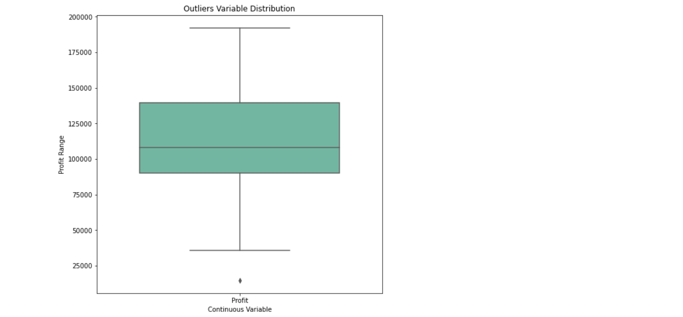
Inference: While looking at the boxplot we can see the outliers in the profit(target variable), but the amount of data is not much (just 50 entries) so it won’t create much negative impact.
State-wise outliers detection
sns.boxplot(x = 'State', y = 'Profit', data = dataset)
plt.show()
Output:
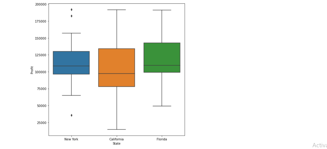
Insights:
1. All outliers presented are in New York.
2. The startups located in California we can see the maximum profits and maximum loss.
Histogram on Profit
sns.distplot(dataset['Profit'],bins=5,kde=True)
plt.show()
Output:
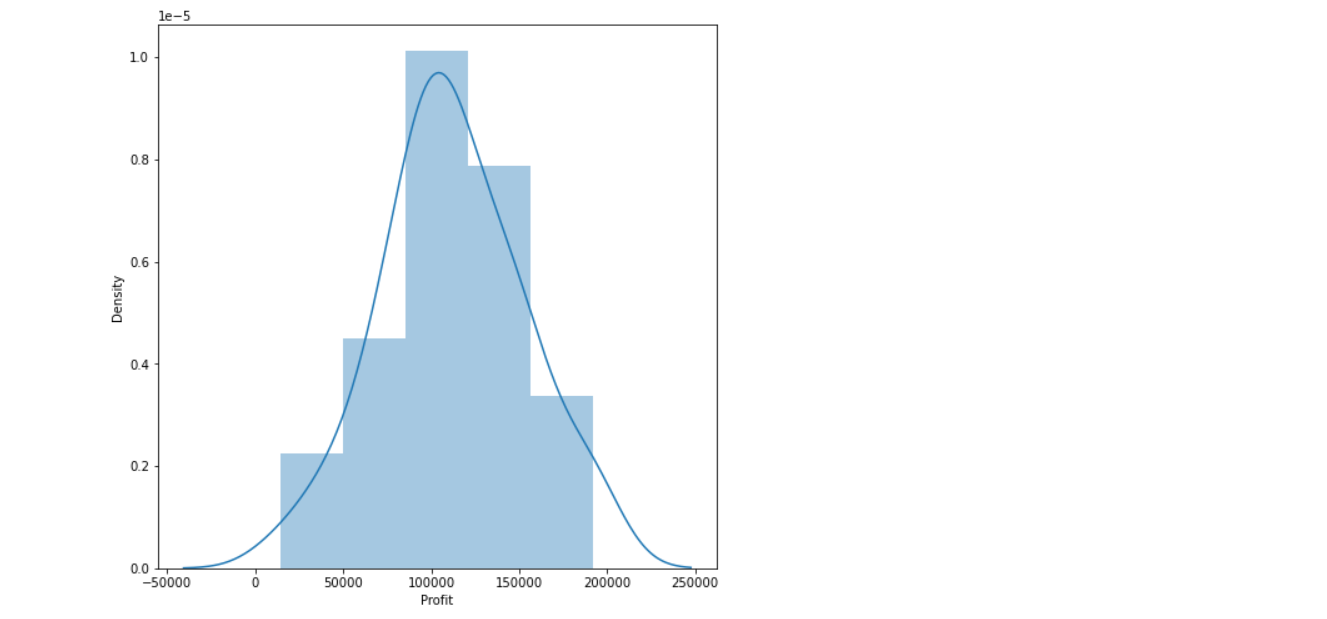
Inference: The average profit (which is 100k) is the most frequent i.e. this should be in the category of distribution plot.
Pair plot
sns.pairplot(dataset)
plt.show()
Output:
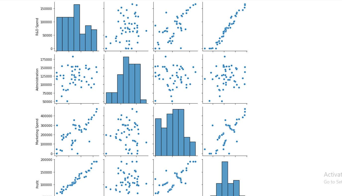
Inference:
- 1. As we can see in the pair pot, Research and development are directly proportional to the investment that we can do.
- 2. The marketing spend seems to be directly proportional (though a little bit outliers are there) with the profit.
- 3. There is no relationship between the second column and profit i.e. our target column.
Model Development
# spliting Dataset in Dependent & Independent Variables
X = dataset.iloc[:, :-1].values
y = dataset.iloc[:, 4].values
Label Encoder
from sklearn.preprocessing import LabelEncoder
Label Encoder: Encode labels with values between 0 and n_classes-1.
labelencoder = LabelEncoder()
X[:, 3] = labelencoder.fit_transform(X[:, 3])
X1 = pd.DataFrame(X)
X1.head()
Output:
Now we have to split the data into training and testing data
from sklearn.model_selection import train_test_split

x_train,x_test,y_train,y_test = train_test_split(X,y,train_size=0.7,random_state=0)
x_train
Output:
array([[130298.13, 145530.06, 323876.68, 1],
       [119943.24, 156547.42, 256512.92, 1],
       [1000.23, 124153.04, 1903.93, 2],
       [542.05, 51743.15, 0.0, 2],
       [65605.48, 153032.06, 107138.38, 2],
       [114523.61, 122616.84, 261776.23, 2],
       [61994.48, 115641.28, 91131.24, 1],
       [63408.86, 129219.61, 46085.25, 0],
       [78013.11, 121597.55, 264346.06, 0],
       [23640.93, 96189.63, 148001.11, 0],
       [76253.86, 113867.3, 298664.47, 0],
       [15505.73, 127382.3, 35534.17, 2],
       [120542.52, 148718.95, 311613.29, 2],
       [91992.39, 135495.07, 252664.93, 0],
       [64664.71, 139553.16, 137962.62, 0],
       [131876.9, 99814.71, 362861.36, 2],
       [94657.16, 145077.58, 282574.31, 2],
       [28754.33, 118546.05, 172795.67, 0],
       [0.0, 116983.8, 45173.06, 0],
       [162597.7, 151377.59, 443898.53, 0],
       [93863.75, 127320.38, 249839.44, 1],
       [44069.95, 51283.14, 197029.42, 0],
       [77044.01, 99281.34, 140574.81, 2],
       [134615.46, 147198.87, 127716.82, 0],
       [67532.53, 105751.03, 304768.73, 1],
       [28663.76, 127056.21, 201126.82, 1],
       [78389.47, 153773.43, 299737.29, 2],
       [86419.7, 153514.11, 0.0, 2],
       [123334.88, 108679.17, 304981.62, 0],
       [38558.51, 82982.09, 174999.3, 0],
       [1315.46, 115816.21, 297114.46, 1],
       [144372.41, 118671.85, 383199.62, 2],
       [165349.2, 136897.8, 471784.1, 2],
       [0.0, 135426.92, 0.0, 0],
       [22177.74, 154806.14, 28334.72, 0]], dtype=object)
Note: Feature Scaling — Useful when Features have different units
“””from sklearn.preprocessing import StandardScaler
sc_X = StandardScaler()
X_train = sc_X.fit_transform(X_train)
X_test = sc_X.transform(X_test)
sc_y = StandardScaler()
y_train = sc_y.fit_transform(y_train)
y_test = sc_y.fit_transform(y_test)”””
from sklearn.linear_model import LinearRegression

model = LinearRegression()
model.fit(x_train,y_train)
print('Model has been trained successfully')
Output:
Model has been trained successfully
Testing the model using the predict function
y_pred = model.predict(x_test)
y_pred
Output:
array([104055.1842384 , 132557.60289702, 133633.01284474,  72336.28081054,
       179658.27210893, 114689.63133397,  66514.82249033,  98461.69321326,
       114294.70487032, 169090.51127461,  96281.907934  ,  88108.30057881,
       110687.1172322 ,  90536.34203081, 127785.3793861 ])
Testing scores
testing_data_model_score = model.score(x_test, y_test)
print("Model Score/Performance on Testing data",testing_data_model_score)

training_data_model_score = model.score(x_train, y_train)
print("Model Score/Performance on Training data",training_data_model_score)
Output:
Model Score/Performance on Testing data 0.9355139722149948
Model Score/Performance on Training data 0.9515496105627431
Comparing the predicted values and actual values
df = pd.DataFrame(data={'Predicted value':y_pred.flatten(),'Actual Value':y_test.flatten()})
df
Output:
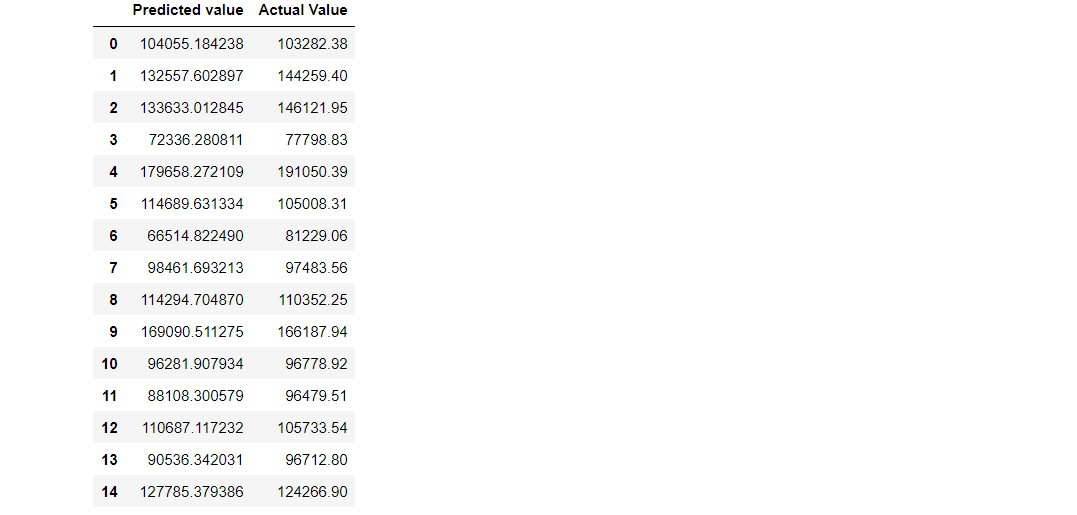
Inference :
As we can see that the predicted value is close to the actual values i.e the one present in the testing set, Hence we can use this model for prediction. But first, we need to calculate how much is the error generated.
Model evaluation
1. R2 score: R2 score – R squared score. It is one of the statistical approaches by which we can find the variance or the spread of the target and feature data.
from sklearn.metrics import r2_score

r2Score = r2_score(y_pred, y_test)
print("R2 score of model is :" ,r2Score*100)
Output:
R2 score of model is: 93.39448007716636
2. MSE: MSE – Mean Squared Error. By using this approach we can find that how much the regression best fit line is close to all the residual.
from sklearn.metrics import mean_squared_error

mse = mean_squared_error(y_pred, y_test)
print("Mean Squarred Error is :" ,mse*100)
Output:
Mean Squared Error is: 6224496238.94644
RMSE: RMSE – Root Mean Squared Error. This is similar to the Mean squared error(MSE) approach, the only difference is that here we find the root of the mean squared error i.e. root of the Mean squared error is equal to Root Mean Squared Error. The reason behind finding the root is to find the more close residual to the values found by mean squared error.
rmse = np.sqrt(mean_squared_error(y_pred, y_test))
print("Root Mean Squarred Error is : ",rmse*100)
Output:
Root Mean Squared Error is: 788954.7666974603
MAE: MAE – Mean Absolute Error. By using this approach we can find the difference between the actual values and predicted values but that difference is absolute i.e. the difference is positive.
from sklearn.metrics import mean_absolute_error

mae = mean_absolute_error(y_pred,y_test)
print("Mean Absolute Error is :" ,mae)
Output:
Mean Absolute Error is: 6503.577323580025
Conclusion
So, the mean absolute error is 6503.577323580025. Therefore our predicted value can be 6503.577323580025 units more or less than the actual value.
Okay, so that’s a wrap from my side!
Endnotes
Thank you for reading my article 🙂
I hope you guys will like this step-by-step learning of the startup’s profit prediction using machine learning. Happy learning!
Here’s the repo link to this article.
Here you can access my other articles which are published on Analytics Vidhya -Blogathon (link)
If you got stuck somewhere you can connect with me on LinkedIn, refer to this link
About me
Greeting to everyone, I’m currently working in TCS and previously I worked as a Data Science Associate Analyst in Zorba Consulting India. Along with full-time work, I’ve got an immense interest in the same field i.e. Data Science along with its other subsets of Artificial Intelligence such as, Computer Vision, Machine learning, and Deep learning feel free to collaborate with me on any project on the above-mentioned domains (LinkedIn).
Image Source
- Image 1: https://assets.website-files.com/5e6f9b297ef3941db2593ba1/5f3a434b0444d964f1005ce5_3.1.1.1.1-Linear-Regression.png


