This article was published as a part of the Data Science Blogathon
Introduction
Hello Everyone, I hope you are doing well. Ever wondered, how great would it be, if we could predict, whether our request for a loan, will be approved or not, simply by the use of machine learning, from the ease and comfort of your home? Sounds fascinating right? Well, in this article, I will be guiding you through that!
This will not only be a practical project, which is applicable in the current times but also will add more to your knowledge of how the system of Loan Approval works.
To ease out your excitement, let me tell you, we will be doing that with the help of a Machine Learning model named the Support Vector Machine.
You see, any bank, approves a loan based on the two most vital points:
1) How risky is the borrower currently, (This is the factor, on which the interest rate of the borrower will depend), and
2) Should they lend the money to the borrower at the given risks?
If both of these conditions give an affirmatory result, the bank proceeds with the loan approval.
A brief about Support Vector Machine Model
The algorithm that we shall be using for this purpose, is the Support Vector Machine. Support Vector Machine,(SVM), falls under the “supervised machine learning algorithms” category. It can be used for classification, as well as for regression. In this model, we plot each data item as a unique point in an n-dimension,(where n is actually, the number of features that we have), with the value of each of the features being the value of that particular coordinate. Then, we perform the process of classification by finding the hyper-plane that differentiates the two classes.
Take a look at the graph below:
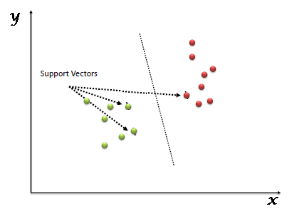
Image source: link
Why choose Support Vector Machine over other algorithms?
You might be thinking the same question. Why SVM, and not the other commonly used algorithms like Logistic Regression, etc. Well, you see there are no such algorithms, which we can strictly say, are better than the other. It all depends on the type of operations we are performing, and the type of data we are dealing with.
SVM is preferred over other algorithms when :
1)The data is not regularly distributed.
2)SVM is generally known to not suffer the condition of overfitting.
3)Performance of SVM, and its generalization is better on the dataset.
4)And, lastly, SVM is known to have the best results for classification types of problems.
Support Vector Machine Project
Now that we are aware of the algorithm that we are going to use, let us plan the tasks that lie ahead of us to achieve the ultimate predictive goals.
Let us divide the tasks, and represent them in a workflow.
It must look something like this :
.png)
Image 1
Now that we are aware of what lies ahead of us, let us complete each of these tasks step by step.
Dataset
The foremost thing that is needed the most, in a machine learning project, is a dataset.
A dataset, as the name says, is a set or collection of data. It contains all the values that we need to work with, to get the necessary results.
For this project, the dataset that I have used is the one I found on Kaggle. You can use any dataset available on the internet that you feel comfortable working with.
The link to the dataset I have used is: link.
Note: You must always keep in mind the fact, that, the more the number of training values present in the dataset, the better will be the prediction that our trained model will be making. Although, a bigger dataset, means that it will consume more time to train the model. So if you are a beginner, I would suggest you, go for the dataset that I have used.
Let’s code!
For this project, I have used python. You can use any python editing environment that you like, eg. PyCharm, Jupyter Notebook, Sublime, Atom, VSCode, etc.
What I have used is a Google Colab Notebook.
The benefit of using a Colab notebook is that we do not need to run anything locally. All the processes are run on the servers of Google. All you need is a stable Internet Connection.
Importing Dependencies :
Let us first import all the modules and libraries that we are going to use in the future while making the project. The dependencies that we will be using are :
numpy, pandas, seaborn, and ScikitLearn.
import numpy as np
import pandas as pd
import seaborn as sns
from sklearn.model_selection import train_test_split
from sklearn import svm
from sklearn.metrics import accuracy_score
When we move on, you will get to know the use of each of these.
Data Collection and Processing
Simply downloading the dataset will not do. We need to link the dataset to our code so that our code can read the data from the table.
The dataset will be in the format of a CSV. Thus to read it, we will be taking the help of the pandas method, called read_csv()
We are strong the dataset in the variable called “loan_dataset”. We can thus now refer to the entire dataset by this variable name.
loan_dataset = pd.read_csv('/content/dataset.csv')
To get a glance at the first 5 rows of the dataset, use the head() method :
import numpy as np
import pandas as pd

loan_dataset = pd.read_csv('train.csv')
print(loan_dataset.head())
.png)
The meaning of the terms in the row headings can be found out on the website, from which we have downloaded the dataset.
Now, let us check the number of rows and columns in the dataset. We run the command :
loan_dataset.shape
It gives the output :
(614,13)
Now, the most important part, let us check, how many values are missing from the dataset. We use the command :
loan_dataset.isnull().sum()
We find: Gender:13
Married: 3
Dependents: 15
Self_Employed: 32
And so on…
Now, thus to get rid of the missing values, let us drop them using the command :
loan_dataset = loan_dataset.dropna()
Now again let us verify whether there are any more missing values left:
loan_dataset.isnull().sum()
No, we find that there are no missing values present in the dataset anymore.
Now what we will do, is called label encoding.
We will be replacing the loan status of ‘Y’ with 1, and ‘N’ with 0, for better reference.
Let us count the frequency of each value in the “Dependent” column:
loan_dataset[‘Dependents’].value_counts()
We find :
0     274
2      85
1      80
3+     41
Name: Dependents, dtype: int64
So we will replace the value of 3+ with 4 to better performance.
loan_dataset = loan_dataset.replace(to_replace='3+', value=4)
Again, what we will do is, convert the categorical columns, to numerical values for better reference.
loan_dataset.replace({'Married':{'No':0,'Yes':1},'Gender':{'Male':1,'Female':0},'Self_Employed':{'No':0,'Yes':1},
                      'Property_Area':{'Rural':0,'Semiurban':1,'Urban':2},'Education':{'Graduate':1,'Not Graduate':0}},inplace=True)
Now when we run :
loan_dataset.head()
We find that all the values have been changed to numerical values.
Splitting Data and Label :
Let us split the data and label into the X and Y variables :
X = loan_dataset.drop(columns=['Loan_ID','Loan_Status'],axis=1)
Y = loan_dataset['Loan_Status']
Thus now, X will store all the features on which the loan status depends, excluding the loan status itself.
Y will store only the Loan Statuses.
Splitting X and Y into Training and Testing Variables
Now, we will be splitting the data into four variables, viz., X_train, Y_train, X_test, Y_test.
X_train, X_test,Y_train,Y_test = train_test_split(X,Y,test_size=0.1,stratify=Y,random_state=2)
Let’s understand each of the variables by knowing what type of values they will be storing :
X_train: contains a random set of values from variable ‘ X ‘
Y_train: contains the output (the Loan Status) of the corresponding value of X_train.
X_test: contains a random set of values from variable ‘ X ‘, excluding the ones already present in X_train( as they are already taken).
Y_train: contains the output (the Loan Status) of the corresponding value of X_test.
test_size: represents the ratio of how the data is distributed among X_trai and X_test (Here 0.2 means that the data will be segregated in the X_train and X_test variables in an 80:20 ratio). You can use any value you want. A value < 0.3 is preferred.
Training our Support Vector Machine model
Let us name the SVM model “classifier“.
Let us define the model:
classifier = svm.SVC(kernel='linear')
Now, let us train our defined model.
classifier.fit(X_train,Y_train)
Now that our model is trained, let us train it with the values of X_train, let us now check its accuracy, by comparing it to Y_train.
X_train_prediction = classifier.predict(X_train)
training_data_accuray = accuracy_score(X_train_prediction,Y_train)
Let us print the Accuracy Score :
print('Accuracy on training data : ', training_data_accuray)
The Accuracy Score came out to be: 0.7986111111111112
Now let us do the same thing with the Testing Values :
X_test_prediction = classifier.predict(X_test)
test_data_accuray = accuracy_score(X_test_prediction,Y_test)
And again let us print the accuracy score :
print('Accuracy on test data : ', test_data_accuray)
The output came out to be :
Accuracy on test data: 0.8333333333333334
Thus it seems our trained model performed better on the testing set than the training set.
Scope of Improvements
Now the thought must have crossed your mind, that how can we improve our results if at all.
Well, let me tell you a few things first.
As you have seen here, our training prediction score was a tad lower, than the testing prediction score. This is okay. Yes, it sounds awkward, but it’s actually fine. You must also be thinking, why did I check the prediction score on the training data at all? Well, to check for a condition, that sometimes arises while training a model in Machine Learning, called as Over-Training.
A short brief of Overfitting is: The model is so poorly trained, that it gives a very high score on the training data (eg: >90%), but gives an extremely low score on the testing data (eg: <15%).
So to check for that, we see the scores for both cases.
Now, coming to the scope of improvements and modifications, We can improve the accuracy score, by doing some of the following, though it is not guaranteed, that the results will change for the better.
1)Taking a bigger dataset with versatile and large training data. But keep in mind while taking a large dataset, the bigger the dataset, the more processing time will the execution take.
2) Checking for various algorithms. There is no such convention, that we must use a specific algorithm, for a specific problem set. We chose the algorithm based on the type of dataset. You might even have to opt for the method of “trial & error”.
3)Optimize the parameters. If you don’t do a grid search for the parameters (C, kernel parameters), it’s a matter of luck if your SVM model does well. The libsvm website has Matlab code explaining this case.
The practicality of this Project
Now let us refer to the elephant in the room. Is the above code ready to be deployed in the banking systems?
A straightforward answer will be NO.
The reasons are:
1) I have used an extremely small dataset. Thus the training dataset is not enough for the model to predict for the various kinds of people that dwell on this earth, with various backgrounds.
2) Real-life scenarios are quite different than what we discuss in theory. There arise many exceptions, that need to be dealt with, and even, the decision-making supremacy, whether a person can be sanctioned a loan or not, cannot be given to a machine that predicts on the basis of these few lines of codes. Humans do have to intervene in those exceptional cases.
But does this mean, all that we did was a sheer waste?
Well, No again. We can use this concept to act as a parallel decision-making feature in the banks, that might be used to second the decisions of the bank people. But it must not be used solely, without the intervention of humans.
End Notes
As you saw in this project, we first train a machine learning model, then use the trained model for prediction. Similarly, any model can be made much more precise and accurate for predictions, by feeding a very large dataset, to get a very accurate and realistic score.
That is it for now.
Thanks for reading…
If you liked the article, do share it with your friends too.
About the Author
Heyy, I am Pinak Datta, currently, a second-year student, pursuing Computer Science Engineering from Kalinga Institute of Industrial Technology. I love Web development, Competitive Coding, and a bit of Machine Learning too. Please feel free to connect with me through my socials. I am always up for a chat with like-minded people.
Till then, Goodbye, and have a good day.
Image Source:
- Image 1: https://www.youtube.com/watch?v=XckM1pFgZmg&list=PLfFghEzKVmjvuSA67LszN1dZ-Dd_pkus6&index=5
Hi, I'm Pinak Datta, currently pursuing my B.Tech in Computer Science and Engineering from Kalinga Institute of Industrial Technology. I'm in my third year of study and I've always had a keen interest in technical writing and software development. I love to develop programs and scripts using Python and have worked on several projects in this language.
Apart from my academic pursuits, I've also participated in various hackathons and coding competitions. These experiences have allowed me to showcase my creativity and problem-solving abilities in the field of computer science.


