This article was published as a part of the Data Science Blogathon.
Introduction
Any company in existence today thrives to make a profit. Insurance companies are profitable when the claims that they issue are lesser than the premiums they receive.
This is the real-world problem we are going to tackle today. If there is a method by which the insurance company can predict a person’s hospital bills, they would be able to generate a financial gain.
This article aims to provide a good starter for someone who wants to solve a real-world problem using classical machine learning.
We have data of about 1338 observations(rows) and 7 features(columns) including age, gender, BMI(Body Mass Index), number of children they have, the region they belong to, and if they are a smoker or a non-smoker. Our task is to uncover a relationship that might exist between a person’s hospital bills and their family conditions, health factors, or location of residence.
With this introduction, we start exploring the data. Remember that garbage in is garbage out. You could use the best possible machine learning model but if your data is garbage your results would not be good as well. This makes it imperative to have a thorough data analysis. Let’s begin.
Data Exploration in Machine Learning
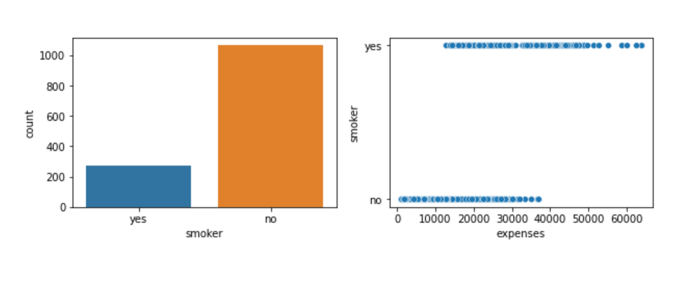 From the count plot on the left, we know that the data has more non-smokers than smokers. Even then from the plot on the right, it is evident that the hospital bills of a smoker are higher than those of non-smokers. We can certainly see a pattern between the feature ‘smoker’ and our target ‘hospital bills’.
Let’s look at the next feature, children (which gives us the number of children a person has)
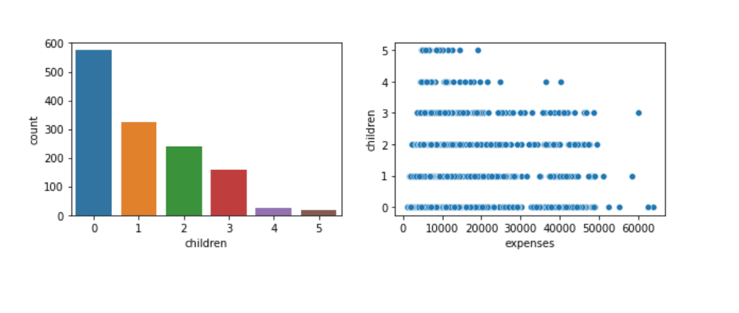
What I thought before plotting the above graphs was an increase in hospital bills with an increasing number of children, but our data do not abide by my initial belief. As you can see from the scatter plot on the right, there are some instances when observations with 0 children have more bills than observations with 5 children. Our data is also imbalanced with respect to the feature ’children’, from the count plot on the left we observe that we have the most observations with people having 0 children and the least with 5 children.
Moving on to further visualize features ‘Age’ and ‘BMI’.
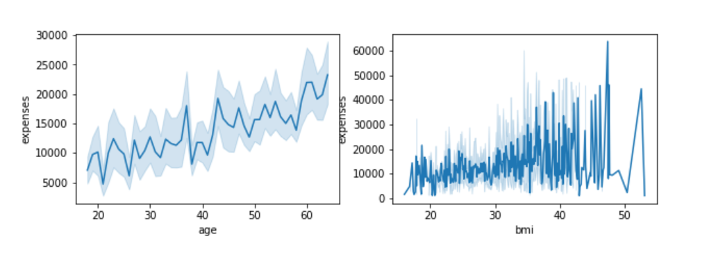
The graph on the left establishes the trend of direct proportionality between age and bills, with an increase in age we can see in most cases an increase in bills.
BMI and expenses line graph on the right does not represent any pattern as we can see some instances of higher BMI with lower expenses, what we can establish for feature BMI is the lowest value in our data is 15 and the highest is up to 60.
The last feature we need to look into is ‘gender’.
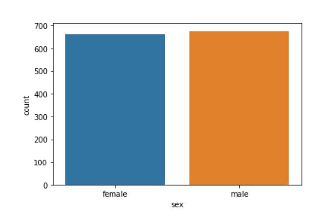
The count plot above shows that we have a good balance in the data as far as gender is concerned. We have an almost equal number of males and females.
For further understanding of the impact of the input features (Age, BMI, region, gender, smoker) on the target variable expenses, we plot a correlation matrix.
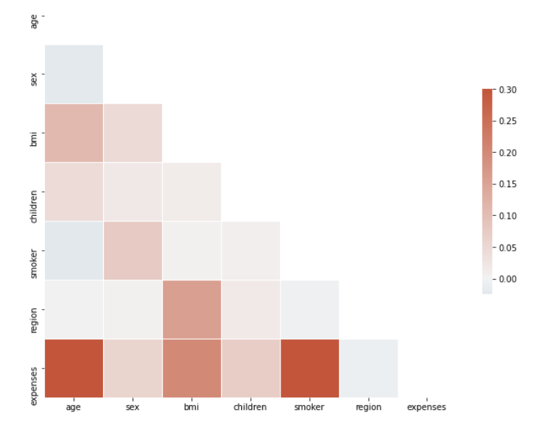
From the correlation matrix above, we establish the following:
The highest correlation can be observed between expenses and age followed by smokers and expenses; BMI and expenses display a good correlation too. Let us further use these to see how they perform to predict hospital bills.
Data Preprocessing in Machine Learning
Before feeding data into the model we would need to do certain checks in other words preprocess the data.
1. Handling missing data (Reference:- https://towardsdatascience.com/7-ways-to-handle-missing-values-in-machine-learning-1a6326adf79e)
The dataset we are working with currently does not have any missing data which is why we do not need to perform this step.
2. Encoding categorical data.
Machine learning models can only work with numerical data, which is why we need to logically encode the categorical features in our dataset to numeric values. There are many ways to perform encoding I am using LabelEncoder from the sklearn library for this case study.
from sklearn.preprocessing import LabelEncoder
label = LabelEncoder()
df.iloc[:,1] = label.fit_transform(df.iloc[:,1])
df.iloc[:,5] = label.fit_transform(df.iloc[:,5])
df.iloc[:,4] = label.fit_transform(df.iloc[:,4])
Above is a code snippet displaying the use of LabelEncoder for encoding categorical features region, smoker, and sex. At the end of this article, I would also link my entire notebook for your reference.
Fitting a Model and Making Predictions
Machine learning involves a lot of experimentation, I tried using a combination of different features and I found that the gender and region features were not contributing much to the target(expense) variable. Considering the same we divide our data frame into X and Y as below.
X = df[['bmi','age','smoker','children']]
Y = df['expenses']
Using sklearn’s inbuilt function train_test_split we divide the data into training and validation data.
Why do we need to divide data into training and validation?
The short answer is to avoid overfitting and to evaluate your model correctly. For a detailed explanation, I suggest you to refer (https://machinelearningmastery.com/train-test-split-for-evaluating-machine-learning-algorithms/)
X_train,X_test,y_train,y_test = sklearn.<a onclick="parent.postMessage({'referent':'.sklearn.model_selection'}, '*')">model_selection.train_test_split(X,Y,test_size=0.25)
Our problem is a regression problem as we are trying to predict expense which is a real-valued number. We would use DecisionTreeRegressor and LinearRegression models for the above task.
from sklearn.tree import DecisionTreeRegressor
from sklearn.model_selection import cross_val_score
regressor = DecisionTreeRegressor(random_state=0)
#cross_val_score(regressor, X_train, y_train, cv=10)
regressor.fit(X_train, y_train)
y_predict = regressor.predict(X_test)
mse_dt = mean_squared_error(y_test,y_predict,squared=False)
print(mse_dt)
6900.60117589873
from sklearn.linear_model import LinearRegression
regressor = LinearRegression()
#cross_val_score(regressor, X_train, y_train, cv=10)
regressor.fit(X_train, y_train)
y_predict = regressor.predict(X_test)
mse_dt = mean_squared_error(y_test,y_predict,squared=False)
print(mse_dt)
5908.41334052373
We get a lower mean squared error with Linear Regression than the Decision tree regressor. We can further lower the MSE(mean squared error) or improve the model performance by using hyperparameter tuning methodologies like Grid Search and Random Search.
Deploying a model. After you are satisfied with your model’s performance you would have to deploy the model such that the intended users can use the functionality.
We would today look at the gradio library that lets us build a web application using just a few lines of code.
!pip install gradio
import gradio as gr

def greet(<a onclick="parent.postMessage({'referent':'.kaggle.usercode.19256245.71583406.greet..bmi'}, '*')">bmi,<a onclick="parent.postMessage({'referent':'.kaggle.usercode.19256245.71583406.greet..age'}, '*')">age,<a onclick="parent.postMessage({'referent':'.kaggle.usercode.19256245.71583406.greet..smoker'}, '*')">smoker,<a onclick="parent.postMessage({'referent':'.kaggle.usercode.19256245.71583406.greet..children'}, '*')">children):
    if <a onclick="parent.postMessage({'referent':'.kaggle.usercode.19256245.71583406.greet..smoker'}, '*')">smoker:
        <a onclick="parent.postMessage({'referent':'.kaggle.usercode.19256245.71583406.greet..is_smoker'}, '*')">is_smoker = 1
    else:
        <a onclick="parent.postMessage({'referent':'.kaggle.usercode.19256245.71583406.greet..is_smoker'}, '*')">is_smoker = 0
    <a onclick="parent.postMessage({'referent':'.kaggle.usercode.19256245.71583406.greet..X_test'}, '*')">X_test = pd.<a onclick="parent.postMessage({'referent':'.pandas.DataFrame'}, '*')">DataFrame.from_dict({'bmi':[<a onclick="parent.postMessage({'referent':'.kaggle.usercode.19256245.71583406.greet..bmi'}, '*')">bmi],'age':[<a onclick="parent.postMessage({'referent':'.kaggle.usercode.19256245.71583406.greet..age'}, '*')">age],'smoker':[<a onclick="parent.postMessage({'referent':'.kaggle.usercode.19256245.71583406.greet..is_smoker'}, '*')">is_smoker],'children':[<a onclick="parent.postMessage({'referent':'.kaggle.usercode.19256245.71583406.greet..children'}, '*')">children]})
    print(<a onclick="parent.postMessage({'referent':'.kaggle.usercode.19256245.71583406.greet..X_test'}, '*')">X_test)
    <a onclick="parent.postMessage({'referent':'.kaggle.usercode.19256245.71583406.greet..y_predict'}, '*')">y_predict = regressor.predict(<a onclick="parent.postMessage({'referent':'.kaggle.usercode.19256245.71583406.greet..X_test'}, '*')">X_test)
    print(<a onclick="parent.postMessage({'referent':'.kaggle.usercode.19256245.71583406.greet..y_predict'}, '*')">y_predict)
    return <a onclick="parent.postMessage({'referent':'.kaggle.usercode.19256245.71583406.greet..y_predict'}, '*')">y_predict[0]

iface = gr.<a onclick="parent.postMessage({'referent':'.gradio.Interface'}, '*')">Interface(
  fn=greet,
  inputs=['text','text','checkbox','text'],
  outputs="number")
iface.launch(share=True)
What we have done in the above code is created a function that takes input from the feature entered by the user and predicts an amount for your hospital expense.
Through gradio, we create an interface that passes the input from the webpage to the function for prediction and displays the function’s predicted output on the webpage. I would recommend you to read the official documentation of gradio before getting started with it (https://gradio.app)
As promised, link to my code.
Conclusion
The key takeaways from the above article are as follow:
1) A simpler model like Linear Regression can perform better than Decision trees for some datasets.
2) Being a smoker or having more number of children increases the possibility of hospital expenses.
About the Author
Hello Everyone!
My name is Alifia G and I am a Data Science Enthusiast.
Please feel free to leave a remark below if you have any questions or concerns about the blog. Thank you.
You can know more about me here!
The media shown in this article is not owned by Analytics Vidhya and are used at the Author’s discretion.


