This article was published as a part of the Data Science Blogathon.
Introduction
In 2017, The Economist declared that “the world’s most valuable resource is no longer oil, but data.”
Companies like Google, Amazon, and Microsoft gather large bytes of data, harvest it, and create complex tracking algorithms. Yet, even for companies that do not specialize in data, the collection and analysis of data can propel them to new heights of prosperity.
However, using that data is easier said than done. Between high costs of data software, labor shortages, IT bottlenecks, etc, today many companies are not in a position to leverage the power of their data.
In addition, employees are expected to work with data to create analyses and reports who are often young and relatively inexperienced analysts and do not have the tools and skills they need to work quickly and accurately.
These, Data Analysts and other Data consumers will often need a tool that allows them to connect to various data sources, create calculations and restructure tables, and can also output data into files and databases. There are many tools available in the marketplace that can do this, but one of our favorites is an open-source, drag-and-drop tool known as KNIME (The Konstanz Information Miner).
What is the KNIME Analytics Platform?
KNIME, the Konstanz Information Miner, is a free and open-source data analytics, reporting, and integration platform. KNIME has been used in various fields like Pharmaceutical Research, CRM, Customer Data Analysis, Business Intelligence, Text Mining, and Financial Data Analysis.
KNIME Analytics Platform is the strongest and the most comprehensive free platform for drag and drops analytics, Machine Learning, and ETL (Extract Transform and Load). With KNIME, there’s neither a paywall nor locked features means the barrier to entry is non-existent.
Using the KNIME Analytics Platform, we can create visual workflows using a drag-and-drop style graphical interface, without coding.
In this guide, we will look at the KNIME Workbench and how we can build our first Knime Workflow using the drag-and-drop feature of the KNIME Analytics platform.
The KNIME suite includes two tools:
KNIME Analytics Platform: This is a desktop-based tool where analysts and developers construct workflows.
KNIME Server: This is enterprise software designed for team-based collaboration, automation, management, and deployment of workflows.
What Can we do With the KNIME Analytics Platform?
It enables the creation of visual workflows via a drag-and-drop graphical interface style that requires no coding. KNIME software can blend data from various sources and shape the data to derive statistics. It can clean data and extract and select features for further analysis. The KNIME platform leverages AI and Machine Learning to visualize data with charts that are easy to understand.
Now, let us look at some of the features that the KNIME Analytics platform provides us that make it unique to use it.
The following are some of the features which make KNIME Platform unique to use.
- Intuitive user interface
- ETL processes
- Machine Learning
- Deep Learning
- Natural Language Processing
- API Integration
- Interactive Visual Analytics
- Import/export of workflows to exchange with other KNIME users.

Start KNIME Analytics Platform
If you haven’t yet installed the KNIME Analytics Platform, you can do the same from the download link.
Why Use KNIME?
Let us now try and understand what makes KNIME a unique platform to use as compared to other platforms. The following are some of the advantages of Using KNIME.
- Open Source: The source code is free to download and access.
- Free to Use: KNIME platform is free to use, and all of its features are available for free except for collaboration extensions are available at a cost.
- Business Intelligence: We can get digestible, actionable data to make informed business decisions. Using Predictive modeling via comprehensive visualizations and summary statistics gives us projections for the best course of action.
- Scalable: KNIME Platform is scalable, meaning it can be used to obtain access to Big Data also; integrations to distributed and multi-threaded data processing allow projects to grow.
- End-To-End Analytics: KNIME platform can be used to handle tasks from scratch to finish without the requirement of integrations. We can also use additional integrations for increasing scale and completing advanced analytics.
- Intuitive User Interface.
- Import/export workflows to exchange with other KNIME Users.
KNIME modules cover a vast range of functionality. Some of them are as below:
I/O: It retrieves data from files or databases.
Data Manipulation: This Module pre-processes the input data by using filtering, group-by, pivoting, binning, normalization, aggregation, joining, sampling, partitioning, etc.
Views: This Module helps in visualizing the data and results through several interactive views.
Mining: This Module uses Mining Algorithms like Clustering, rule induction, Decision Tree, Association Rules, Naive Bayes, Neural Networks, Support Vector Machines, etc., to better understand your data.
Hiliting: It ensures that hilted data points in one view are also hilited in other views.
Nodes and WorkFlows
Before we work with our First KNIME workflow, let us look at Nodes and their workflows in detail to understand how the nodes in the KNIME Analytics Platform will perform individual tasks. Each node is a colored box with input and output ports. These Nodes can perform all sorts of tasks like reading/ writing files, transforming data, training models, creating visualizations, etc.
The following is the Node Diagram wherein we can see that it has got a Node Name, Input Port is for the data to be processed, and the output nodes are for the resulting data. Each node has specific settings, which we can use /adjust in a configuration dialog. Only ports of the same type indicated by the same color can be connected.

A traffic light shows the node’s status as in the diagram below.
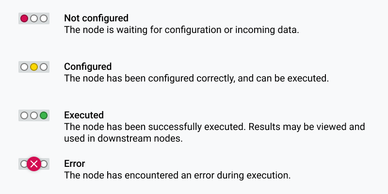
KNIME NODE STATUS
Building our First KNIME Workflow:
Now, let us look at how we can process, analyze and visualize some data by building our First KNIME Workflow. We will build our KNIME workflow where we will read, transform and visualize sales data. The link to download the dataset.
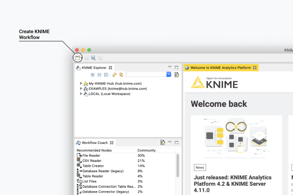
CREATING A WORKFLOW IN KNIME
Once the file is downloaded, open the Analytics Platform and create a new, empty workflow by clicking “New” in the toolbar, as can be seen in the diagram above. Once you click on the new KNIME workflow, a new KNIME workflow will be created, as shown below.
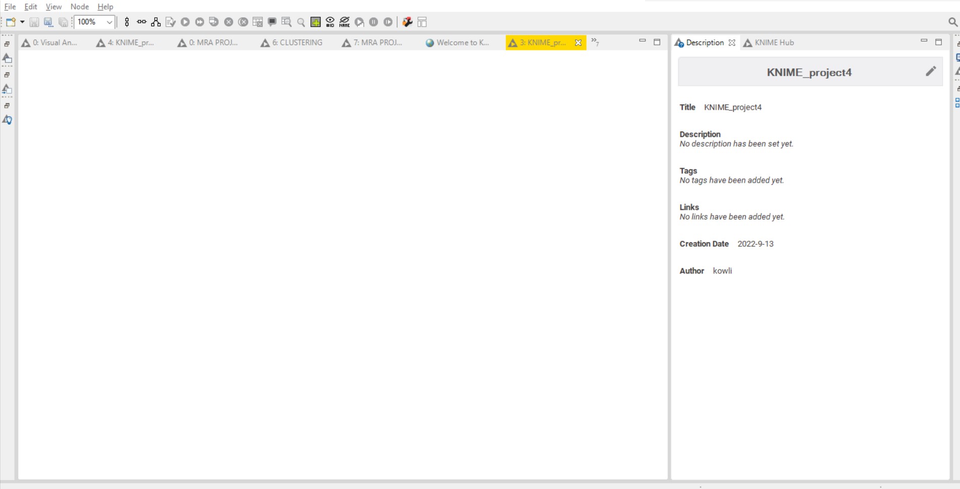
NEW KNIME WORKFLOW
STEP 1: Drag and drop CSV file into workbench editor
From the download folder, drag and drop the CSV file downloaded from the above link into the workbench editor. A File Reader node as seen in the below screenshot will appear on the workflow editor, and its configuration dialog will pop up as can be seen in the below image.
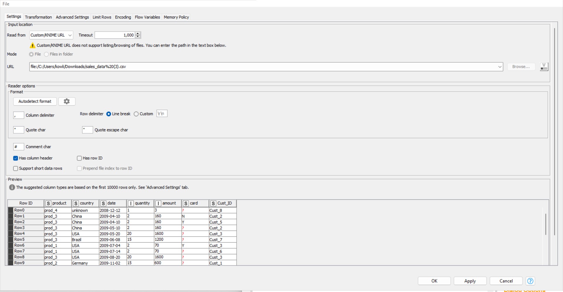
KNIME WORKBENCH
In the above configuration dialog box, click on apply. Once you click on apply a CSV Reader Node as can be seen in the diagram below can be seen.
Right-click on the CSV reader Node and click on Execute. This will read the data from the CSV file, and the Node will be ready with the output file for further processing. To view the output right, click on the executed node and select the File Table option to view the output table.
STEP 2: Filter Data With The Filter Node:
To filter the columns out from the data, we can use the Filter Node available in the column filter node in the search field, as can be seen in the screenshot below. Type Column filter node in the search field, then drag and drop the node to your workflow editor. Connect its input port with the output of the first node, i.e., File Reader Node.
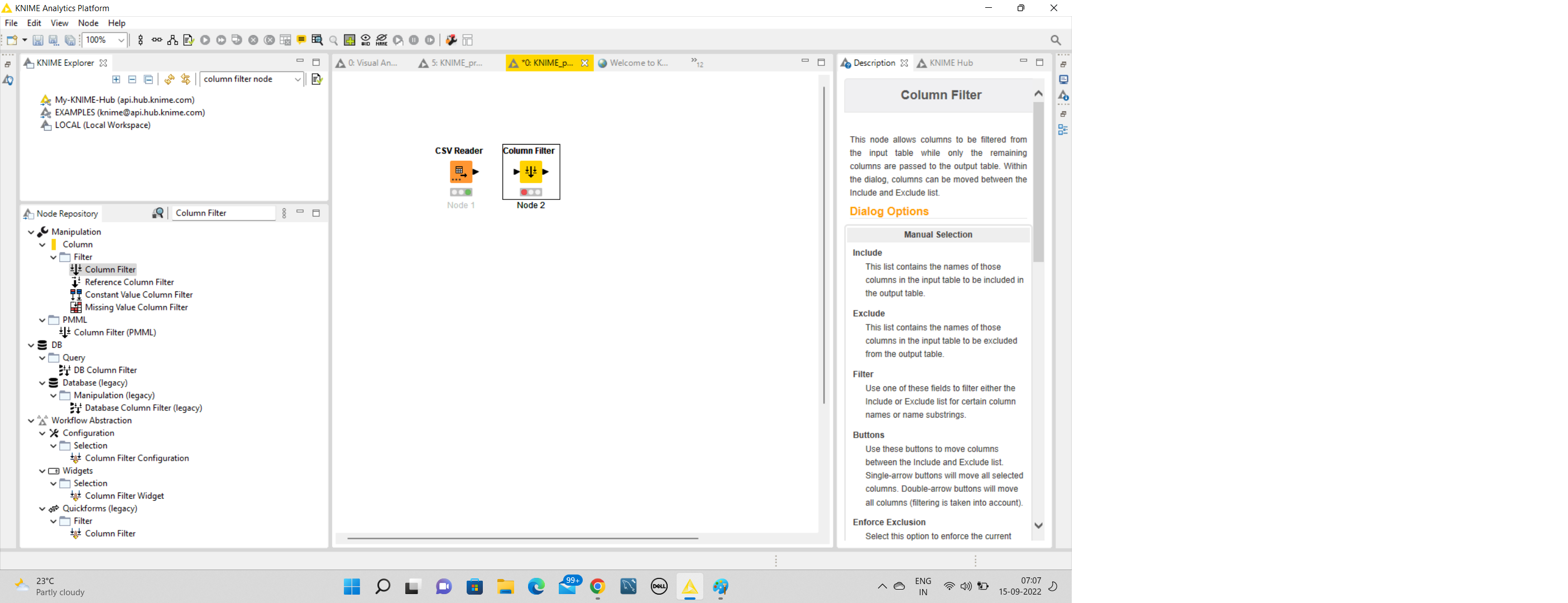
FILTER NODE
To open the configuration dialog, right-click on the node and choose Configure. Now, move the columns ‘country’, ‘date’, and ‘amount’ into the include field available on the right side of the dialog, then click Ok. After executing the node, the output data is available at the output port of the column filter node.
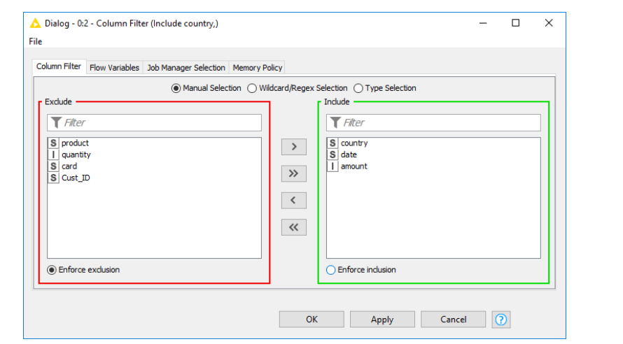
COLUMN FILTER NODE CONFIGURATION DIALOG BOX
STEP 3: Exclude Unknown values with Row Filter Node:
Now, to clean up our data by filtering out rows, we are using the Row Filter Node. Search for the Row Filter Node in the node repository on the left, drag and drop it to the workflow and connect the output of the column filter node to the input of the Row Filter Node.
Open the Row Filter node configuration dialog and exclude rows from the input table where the column ”country”‘ has the value ”unknown” as seen in the screenshot below. Now click OK and execute the node. Now, the filtered data is available at the output of the Row Filter Node.
STEP 4: Visualize your Data with Stacked Area Chart and pie/ Donut Chart
Now, we will try and visualize the data by building a stacked area chart and a pie chart, using the nodes Stacked Area Chart and Pie/ Donut chart. We will now search for the Pie Chart and Stacked Area Chart and add them to the workflow by connecting both to the Row Filter Node. Now configure the column date as the x-axis column in the configuration dialog of the Stacked Area Chart node.
Now, configure the column ”country”‘ as the category column, ”Sum” as the aggregation method, and ”amount” as the frequency column in the Pie/ Donut Chart node. The output is as below.
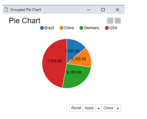
PIE CHART OUTPUT
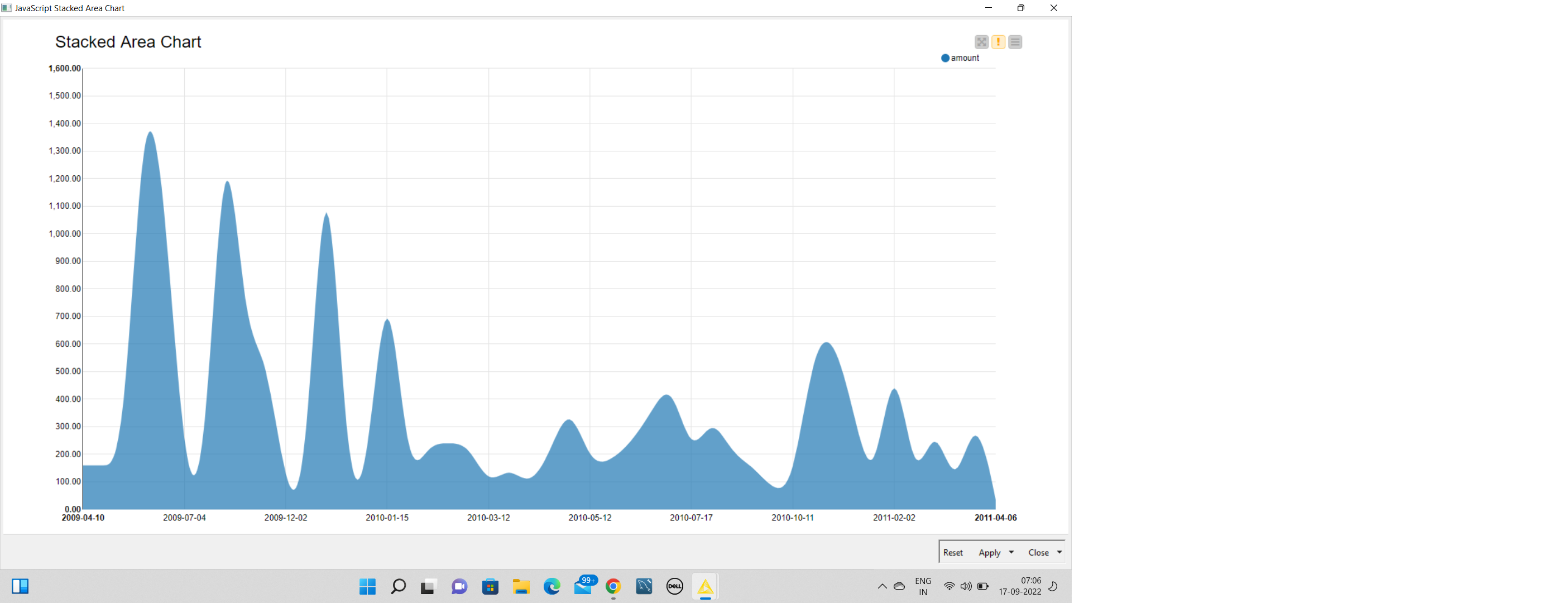
STACKED AREA CHART
Working with Different Data Sources in KNIME
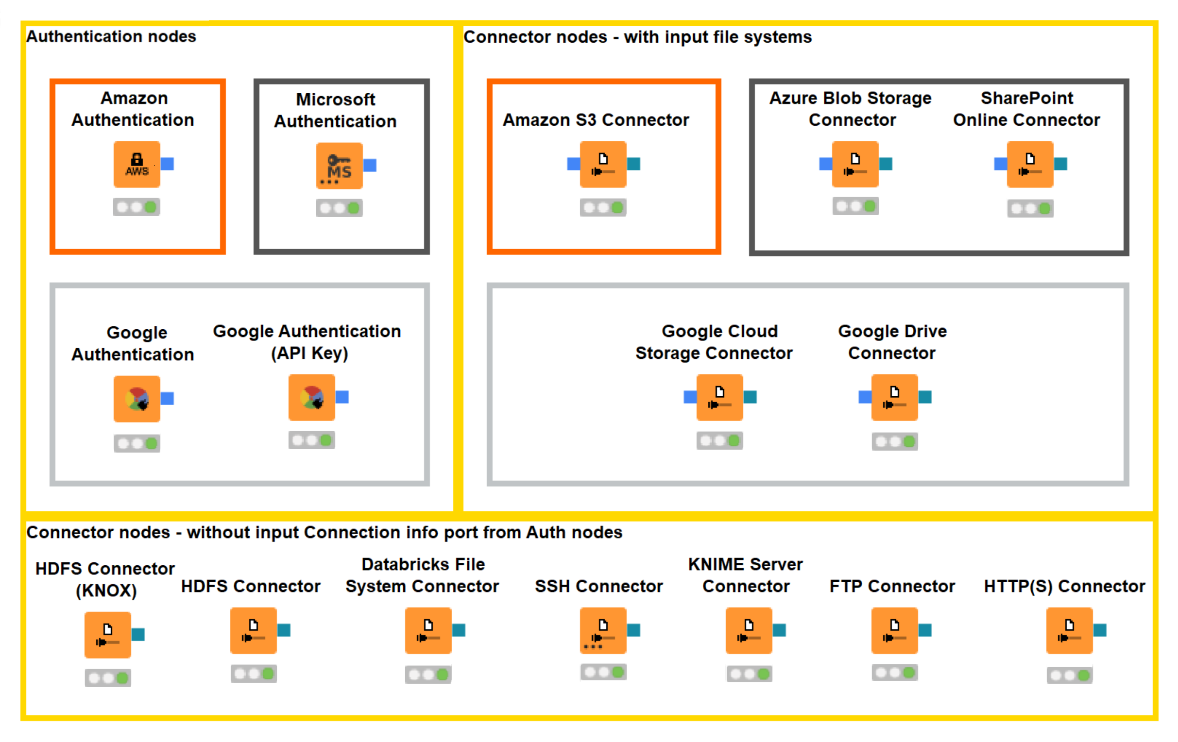
We will look at working with different file systems like Standard File Systems and Connected File Systems, which require a dedicated connector node. KNIME provided connectors for all major cloud platforms such as Azure, Databricks, Amazon, Google, etc. KNIME supports the mixing and matching of different file systems within the same workflow. The following are two different File Systems that the KNIME supports for connecting the data.
Standard File Systems: Standard File Systems are available at any time, i.e., they don’t require a connector node to connect to them. To use a reader node to read a file from a Standard File System, drag and drop the reader node. For example, if you want to read a CSV file, drag and drop an Excel Reader Node from the Node Repository.
Connected File Systems: Connected file systems require a dedicated connector node that allows users to connect to all major cloud platforms such as Azure, Google Cloud, Databricks, and Amazon cloud. This new File handling Framework enables standardized and easy access to both standard and connected file systems. We can read files directly from all supported connected file systems without needing to download them locally.
DIFFERENT NODES IN KNIME
KNIME FILE HANDLING FRAMEWORK FOR AMAZON S3 WITH AZURE BLOB
Amazon S3 meets MS Azure Blob Storage
Now, let’s leave the ground and move into the clouds! When we talk about clouds, two options come to mind: the Amazon Cloud and the MS Azure Cloud. Amazon cloud uses the S3 data repository, and MS Azure uses the Blob Storage data repository.
Now, let’s suppose that we have ended up with data on both clouds, i.e., Amazon cloud and MS Azure Cloud. How could we make two clouds communicate to collect all the data in a single place and analyze it? We know that the clouds rarely talk to each other. Our challenge is to force Amazon Cloud and the MS Azure cloud to communicate and exchange data i.e, we want to blend data from two different clouds and also in the process, we will also try and put a few excel files into the blender, as data analytics process has to deal with an Excel file or two.
The nodes required here are the Connection and the File Picker Nodes, i.e. the Amazon S3 Connection node and the Amazon File Picker node for one cloud service and the Azure Blob Store Connection node and the Blob Store File Picker node for the other cloud service.
From Amazon S3:
First, the Amazon S3 connection node needs to be connected to the Amazon S3 Service by using the credentials and hostname. Next, by using the Amazon S3 File Picker node we will build the full path of the resource selected on S3 and export it as a flow variable. Lastly, the File Reader node uses the content of that flow variable to overwrite the URL of the file to be read, therefore accessing the file on the Amazon S3 Platform.
From MS Azure Blob Storage:
Similar to Amazon S3, we have dedicated nodes for M.S. Azure Blob. Firstly, by using the Azure Blob store connection node we will connect to the Azure Blob Storage Service by using the credentials and hostname provided in its configuration window. The Azure Blob Store File Picker node builds the full path of the resource selected on Blob Storage and exports it as a flow variable, The content of this flow variable is used by the File Reader node to overwrite the URL of the file to be read, thus accessing the file on the Azure Blob Storage platform.
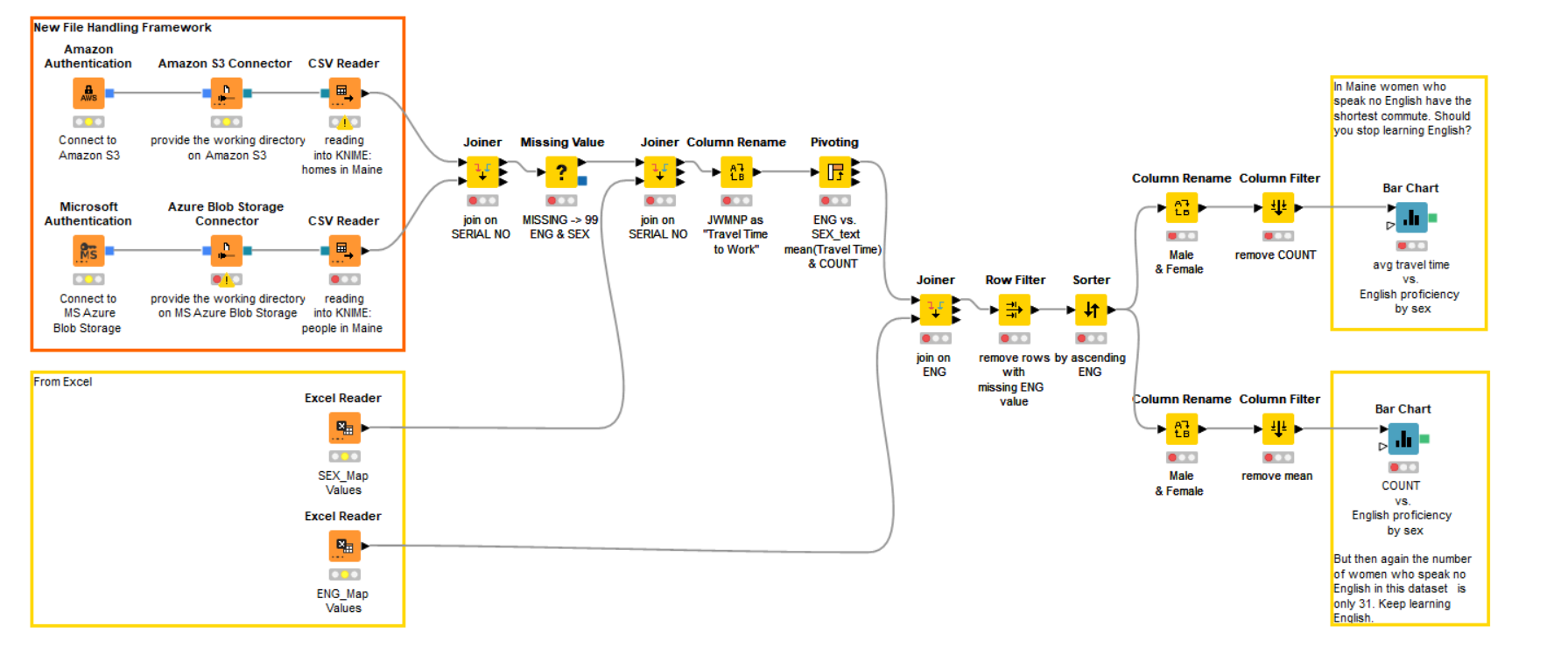
Now, both the data sets are available as data tables in the KNIME Workflow. The following is the workflow image for Blending the Amazon S3 with M.S. Azure Blob storage and a few excel files.
BLENDING OF MS BLOB STORAGE WITH AMAZON S3 AND A FEW EXCEL FILES
The ss13pme.csv contains several randomly interviewed people in the state of Maine, and ss13hme.csv includes information on the house in which the interviewed people live. The interviewed people in both the files are uniquely identified by the Serial Number attribute and then the two datasets are joined using SERIAL Number.
These two data sets can be downloaded from the below link.
http://www.census.gov/programs-surveys/acs/data/pums.html.
Similarly, the data dictionary can be downloaded from the below link.
http://www2.census.gov/programssurveys/acs/tech_docs/pums/data_dict/PUMSDataDict15.pdf
Here, we have concentrated on the attributes like ENG (Fluency in English, Gender, and JWMNP (which is the Travel time to work). The idea here is to identify if there is any interesting pattern across such features in the dataset.
Missing Values in these features are substituted with the Mode of the particular Column. The feature JWMNP is renamed as ‘Travel Time to Work. Now a pivoting node is used to build the two matrices: avg(JWMNP) of ENG vs. Gender and count of ENG vs. Gender.
The codes (1,2) in the Gender attribute are mapped respectively to Male and Female. Similarly, ENG codes (1,2,3,4) are mapped to text which describes fluency in the English Language. A javascript Bar chart node displays the average travel time for females and males depending on their English Proficiency. Another Javascript Bar chart node displays the number of people for each group of males/females and their fluency in the English language.
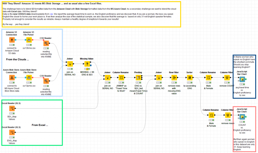
The following workflow blends data from Amazon S3 and MS Azure Blob Storage.
The following workflow blends the data from Amazon S3 and MS Azure Blob Storage. As a bonus, it also throws in some Excel data as well.

BLENDING WORKFLOW OF MS Azure Blob storage with Amazon S3.
Now, after blending the data from Amazon S3 and the data from the Azure Blob storage using the above workflows in KNIME, we were also able to isolate different groups based on their gender and fluency in English. The output can be seen in the plots below.
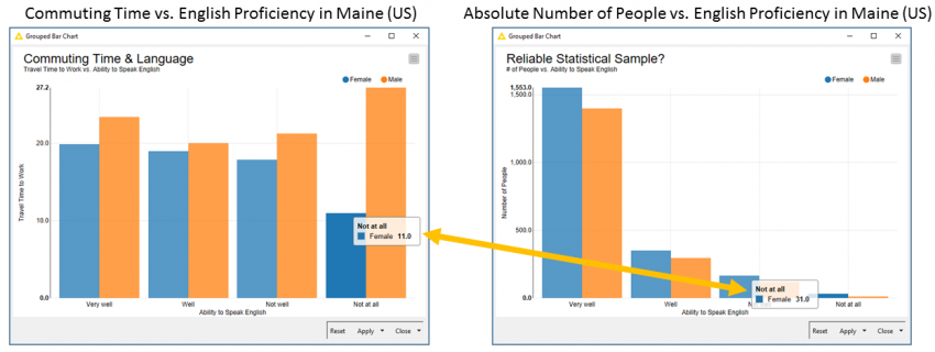
The plot on the left shows us the Average Commuting Time vs. English Proficiency in Maine (U.S.). The plot displays the Absolute Number of People vs. English Proficiency in Maine (U.S.) on the right.
From the above plots, we can see that if a person is a Woman in Maine and Speaks no English, then your commute to work seems to be much shorter than the commute of another woman who speaks better English. Similarly, for a male who does not speak good English, the travel time is relatively very high, as seen from the plot above.
Building a Customer Churn Prediction Model Using KNIME
Now, we will look at building a customer churn prediction model using the KNIME Analytics platform. ‘Churn’ refers to the customer who cancels a contract or a service at the moment of renewal of the service/ contract. Identifying which customers will churn or are at risk of churning is vital for companies to take measures to reduce the churn.
Now, we will build a classic churn prediction application using KNIME, wherein the application consists of two workflows a training workflow in which the model is trained on a set of past customers to assign a risk factor to each one and a deployment model in which that trained model assigns a churn risk to new customers. The following two workflows will do the same in KNIME, which can be seen below.
The data set used in this model is available on Kaggle and can be downloaded from the below link.
https://www.kaggle.com/datasets/becksddf/churn-in-telecoms-dataset
Before going ahead with the model building using KNIME, let us look at the Data Set in some detail to understand its features and understand which features help us in better prediction of the churn.
We have features like International Plan activated or not, total day minutes, total day calls, total day charge, total eve minutes, total eve calls, total eve charge, and similarly for the night as well, which can be used for churn prediction. We also have a column/ feature which says whether the customer has churned in the past or not, which can be used to train our model better.
Now, we will split the dataset into a CSV file Training Dataset (which contains operational data, such as the number of calls, minutes spent, etc.), and an Excel file (which will have the contract characteristics and the churn flag i.e. whether a contract was terminated or not). Our dataset has data for 3,333 customers with 21 features.
Preparing and Exploring the Customer Data:
Step 1: Reading the Data
Now, let us prepare the Dataset for Training. The training workflow is as below. It starts by reading the data; files can be dragged and dropped into the KNIME workflow. We are using the XLS and CSV files, as discussed above.
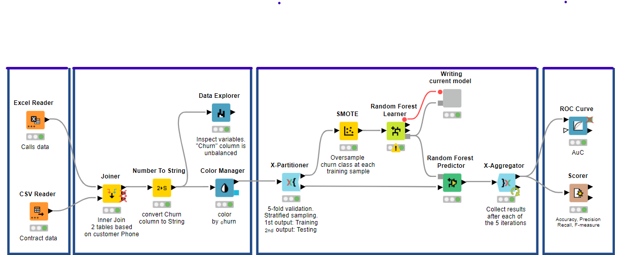
MODEL TRAINING WORKFLOW TO ASSIGN THE CHURN RISK
The above workflow is an example of how to train a Machine Learning Model for a Churn Prediction Task. Here we are training a Random Forest Model after oversampling the Minority class, i.e., Churn Class, with the SMOTE algorithm. We are also using the cross-validation procedure for a more accurate and reliable estimation of the Random Forest Performance.
Step 2: Joining the data from two files:
In this step, we will be joining the data from the same customers in the two files by using their telephone numbers and area codes which are common using the Joiner Node, as can be seen in the workflow above.
Step 3: Converting Churn Column into string type:
In this step, we are going to convert the “Churn” column into string type with the Number to String node to meet our requirement for the upcoming classification algorithm.
Step 4: Exploring the Dataset:
Now, let us further explore the dataset with some visual plots of some basic statistics by using nodes like the Data Explorer node, which calculates the average, variance, skewness, kurtosis, and other basic statistical measures and it also draws a histogram for each of these features in the dataset.
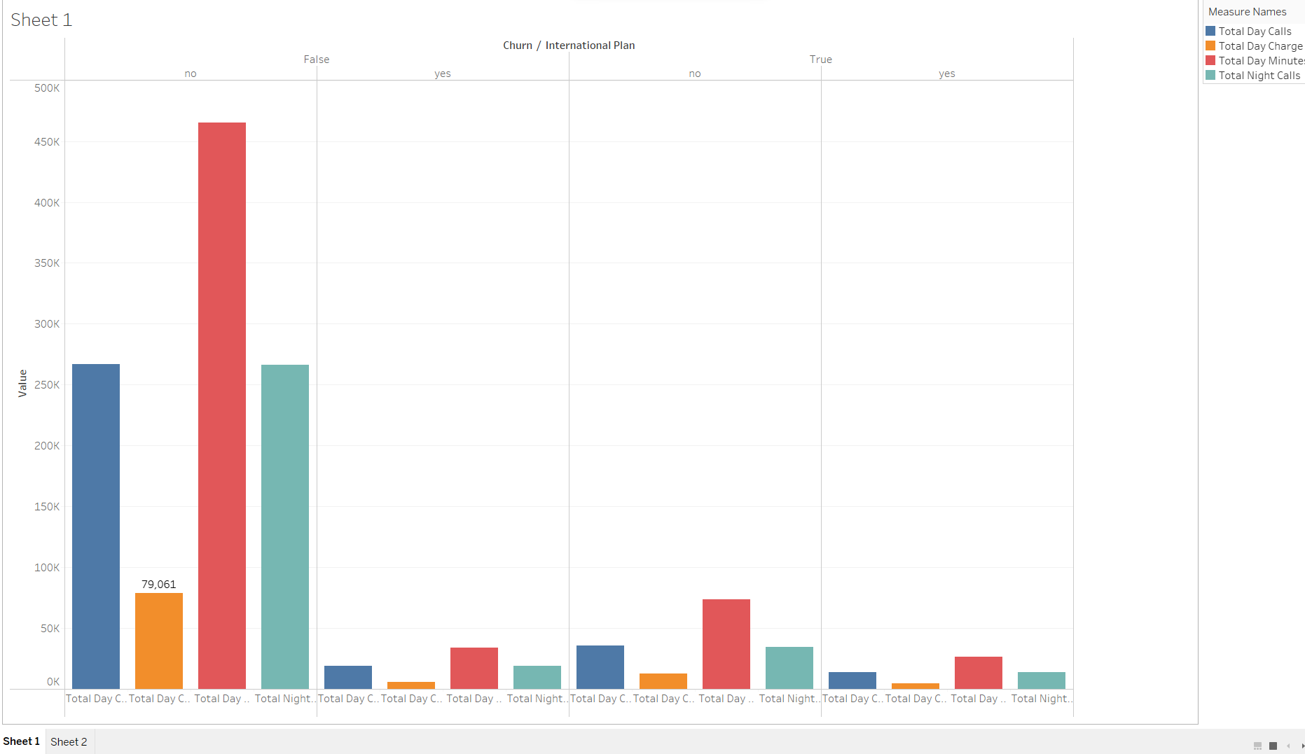
HISTOGRAM REPRESENTING THE CHURN OF THE DATASET. USING TABLEAU.
By viewing the above Histogram plot of the dataset, we can see that the dataset is imbalanced, i.e., most of the observations pertain to the non-churning customer, which is about 85%. To overcome this class imbalance in our dataset, we will use a technique called SMOTE (Synthetic Minority Oversampling Technique) by using SMOTE node in the KNIME node repository. You may learn more about the SMOTE technique here.
https://machinelearningmastery.com/smote-oversampling-for-imbalanced-classification/
Step 5: Training and Testing our Model:
In this step, we will divide our dataset into a Training data set and a Testing dataset and feed the Training dataset into the model for training purposes. We will later test the model using the Test dataset. We chose the Random Forest algorithm implemented by the Random Forest Learner node, with 5 as the minimum node size and 100 trees. The minimum node size is nothing, but it is the basis for node splitting in other words, it will control the depth of the decision trees, while the number of trees will control the model’s bias. Random Forest is chosen as it will offer the best compromise between complexity and performance.
Here the Random Forest Predictor node will rely on the trained model to predict the patterns in the testing data. These predictions will then be consumed or given as input to an evaluator node, like a Scorer node or a ROC node, to estimate the quality of the trained model.
To increase the reliability of the model predictions, the whole learner-predictor block will be inserted into a cross-validation loop, starting with an X-Partitioner node and ending with an X-Aggregator node. The Cross-Validation was set to run a 5-fold validation, meaning it divided our dataset into five equal parts. Each iteration used four parts for training (i.e., 80% of the data for training) and one part for testing (i.e., 20 % of the data for testing). The X-Aggregator node collects all predictions from the test data on all five iterations.
The Scorer node matches the random forest predictions, i.e., output from the Random Forest Predictor node with the original churn values from the dataset. It assesses the model using the evaluation metrics such as Accuracy, Precision, Recall, and F1- Score. The ROC node will then build and display the associated ROC curve and calculate the Area Under the Curve (AUC), a metric for model evaluation.
The Scorer node will match the Random Forest predictions with the dataset’s original churn values and assess model quality using evaluation metrics such as Accuracy, Precision, Recall, and F-measure. The ROC node builds and displays the ROC curve associated with the predictions and then calculates the Area under the Curve (AUC), a metric for model quality. All these metrics range from 0 to 1; the higher the values, the better the models. We obtained a model with 93.8% overall accuracy and 0.89 AUC for this example.
Deploying the Model
Now, as the model has been trained and evaluated and the results are satisfactory, we will deploy the model and apply it to the new data for real churn prediction with data from the real world. The deployment workflow is as below.
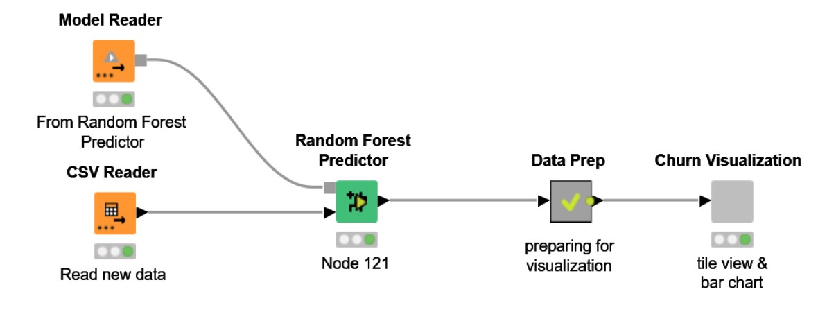
IMAGE 18: MODEL DEPLOYMENT
The best-trained model, which in our case turned out to be from the last cross-validation iteration, and data from new customers are acquired using a CSV Reader node. A Random Forest Predictor node applied the trained model to the new data from the CSV Reader node and produces the probability of churn and the final churn predictions for all input customers. The churn visualization node is used to visualize the data using a Bar Chart or a Pie Chart. The Visualization chart is as below.
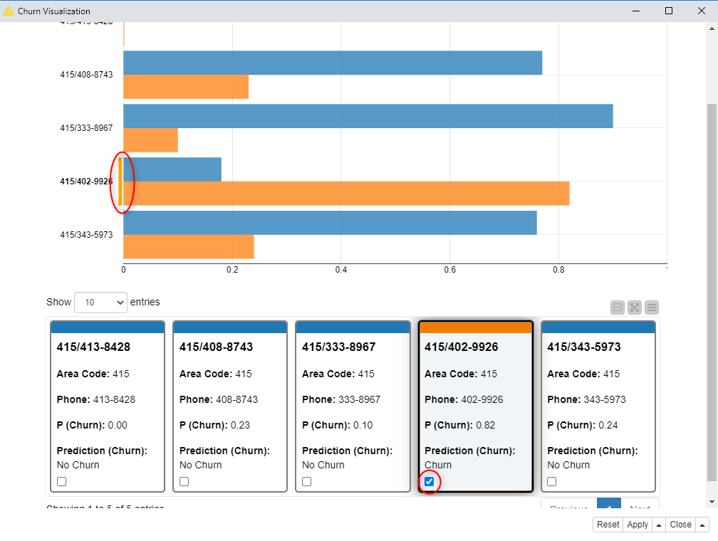
DASHBOARD REPRESENTING THE CHURNERS AND NON-CHURNERS
From the above plot, we can see that the churn risks are associated with orange colored bar chart where the blue-colored bar chart represents the non-churners.
Now let us also look at Some of the Pros and Cons of Using KNIME.
Pros of Using KNIME
- No License Fee.
- Easy to Understand and Learn
- Open Architecture
- No coding is required to execute workflows; advanced excel knowledge is sufficient.
- Good Community support for your Q&A.
- Large data set processing
- Data Manipulation
- Server-based execution.
- Unified interface for data and cleansing.
- Cross-platform interoperability.
The following are some of the Cons rather challenges of Using KNIME.
Cons of Using KNIME
- Cumbersome UI
- Slow to Load.
- KNIME workflows are very big, even for building a straightforward one, due to caching and GUI.
- KNIME’s performance on visualization is not very effective though it has been better on newer versions of KNIME.
- Knowledge of R/ Python is required to use the Statistical analysis in KNIME fully.
- Memory Usage is a challenging area sometimes while using the KNIME platform.
Conclusion
In this article, we tried to understand one of the best tools used for Data Analytics, i.e., KNIME, we also tried and understood its various features, and we built our first KNIME workflow using the drag and drop feature KNIME is known for. Also, we worked with different data sources using KNIME and looked at how to club data from two different clouds using KNIME, i.e., MS Azure Blob storage with Amazon S3.
Also, we have looked at building a Customer Churn Prediction model using the KNIME platform and also looked at the workflow of how to deploy the same.
This brings us to the end of this simple yet comprehensive guide on using KNIME for Data Analysis. This guide aims to provide an in-depth yet simple way of using the KNIME. I did enjoy writing this article and hope the same from readers of this guide and would love to have your feedback in the comments section below.
For further discussion or feedback, feel free to connect with me on my Linked In.
https://www.linkedin.com/in/sumanthkowligi/
The media shown in this article is not owned by Analytics Vidhya and is used at the Author’s discretion.


