Building Customer Churn Prediction Model With Imbalance Dataset

Introduction

The digital revolution is taking place at a very fast pace. Data generation over the cloud is increasing in massive amounts regularly, and data being king in the digital era can win anything. The amount of data is insufficient until it does not reflect or we cannot find meaningful information that can drive business decisions. Data analysts and scientists spend almost 70 percent of their time forming quality data or refining it. Most of the time, data only contains one class of data, and the other class has almost zero presence in the data, known as a class Imbalance problem. There are different ways to deal with a class imbalance dataset that we will learn in this article. 

Learning Objectives

1. Why is the quality of data important in Machine Learning?
2. What is Imbalance Dataset, and How to deal with class Imbalance?
3. Use different Models to control Internally the Imbalance Dataset
4. Measure the accuracy of the Imbalance dataset with perfect performance Metric.
5. Build Customer Churn Prediction model with decent accuracy.

 This article was published as a part of the Data Science Blogathon.

Table Of Contents

1. Brief Introduction to Imbalance Datasets
2. Describing the Dataset
3. Small Talk on Churn Analysis
4. Choosing the Best Performance Metrics
5. Performing Exploratory Data Analysis
   5.1. Explore Target Variable
   5.2. Explore Numerical and Categorical Features
6. Learning to Use Famous Trio Models with Class Imbalance Dataset
   6.1. Applying Cat Boost Algorithm
   6.2. Applying Light GBM
   6.3. Applying XGBoost Algorithm
7. Comparison of Different Models
8. Conclusion

Brief Introduction to Imbalance Datasets

Machine learning operates completely on the data. If data is improper, then model performance will suffer. Consider a scenario where you have bank transaction data. The sample data are shown below, where No states the transaction, which is not fraudulent, and YES states the fraudulent transaction.

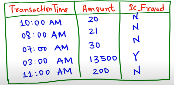
In the above example, the no becomes 80 percent, and the yes becomes 20 percent, so this kind of scenario is called an imbalanced class problem because your model creates a bias toward the more weightage class. The thing of our interest is to understand more fraud transactions, but since we don’t have enough sample data, machine learning models will be unable to learn the pattern of fraud transactions. This is a very common problem in the IT industry while dealing with data. Here we have seen an example of 80-20 percent. You can get different ratios 90:10, 95:5, or even 99:1.

Describing the Data

The dataset we will use is the Customer churn prediction dataset of 2020. It is all about measuring why customers are leaving the business or stating whether customers will change telecommunication providers or not is what churning is. The dataset contains 4250 samples. Each sample has 19 input features and 1 boolean target variable, which indicates the class of the sample.

The dataset is imbalanced, where 86 percent dataset is not churned, and only 14 percent of the data represents churn so our target is to handle the imbalance dataset and develop a generalized model with good performance.

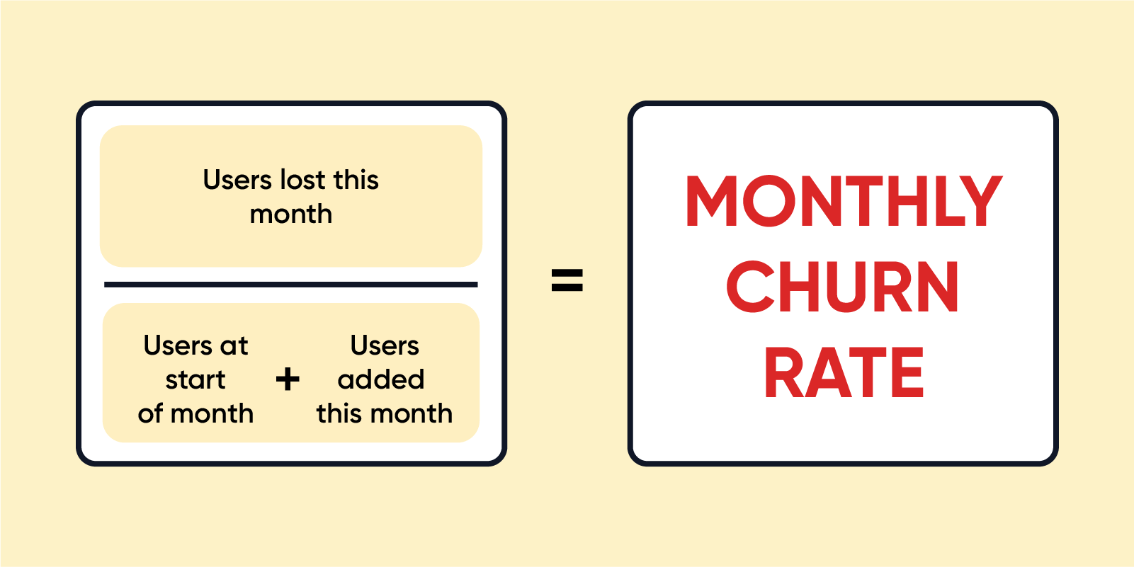
Small Talk on Churn Analysis

Churn Analysis describes the company’s customer loss rate. Churn means Attrition in simple words, which occurs in two forms customer attrition and employee attrition. When the attrition is high, the company’s growth graph starts coming down, and the company suffers a high loss time during the attrition. Churn can be minimized by analyzing the company’s work environment, product growth, market conditions, dealer connections, etc. If churn increases by only one point, then it directly affects the business in a negative perspective. High Churn rates compound very fast that can have a massive loss to the company, so it is important to calculate churn regularly.

Choosing the Best Performance Metric

Since our target variable has imbalanced dataset, we will not use the accuracy score. The recall is used in an imbalance class problem with two classes, which quantifies the number of correct predictions of positive made out of all positive predictions. The formula to find recall is the total number of true positives divided by the total number of true positives and false negatives.

Precision is another choice of metric which calculates accuracy for the minority class. Maximizing the precision will reduce the false positives, while maximizing the Recall will reduce the false negatives. So, according to our problem statement, we must focus on reducing the false negative. Hence we will go with Recall as a performance metric.

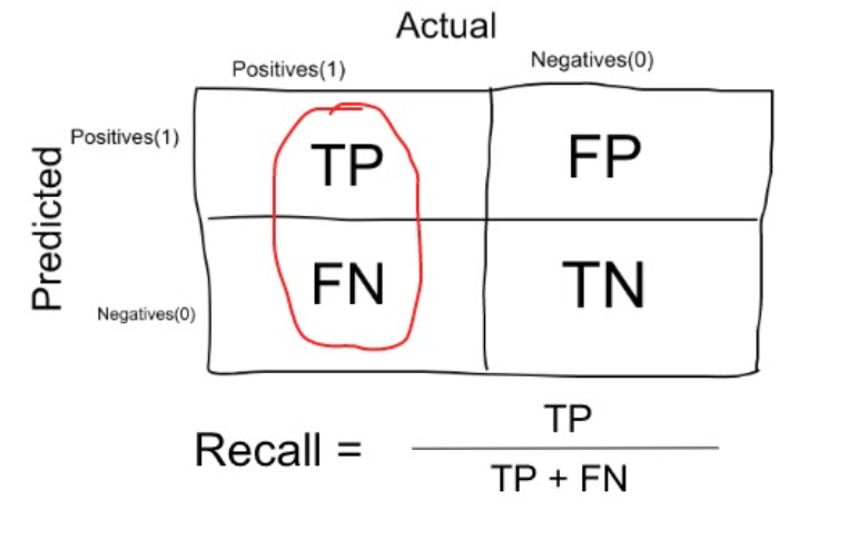
Source: Medium

Performing Exploratory Data Analysis

The first step is to import all the libraries and load the data to explore the data and understand some insights and relationships to take further action on the dataset. We have imported data analytics libraries and data visualization libraries.

Python Code:

import numpy as np
import pandas as pd

df = pd.read_csv('train.csv')

df1 = df.copy() #create copy so preserve original

print(df1.head())

import matplotlib.pyplot as plt
import seaborn as sns
#importing plotly and cufflinks in offline mode
import cufflinks as cf
import plotly.offline
cf.go_offline()
cf.set_config_file(offline=False, world_readable=True)
import plotly 
import plotly.express as px
import plotly.graph_objs as go
import plotly.offline as py
from plotly.offline import iplot
from plotly.subplots import make_subplots
import plotly.figure_factory as ff

pd.set_option('max_columns',100)
pd.set_option('max_rows',900)
pd.set_option('max_colwidth',200)

If you check the null or duplicate values, the result is 0 for each column. So, from the Preliminary analysis, we can conclude some results.

• We will create models with the famous trio XGBoost, Light GBM, and Catboost that predict behavior to retain customer data and develop a focused customer churn prediction.
• For Catboost, types of columns with integers will be converted to float type.
• We have to look at the cardinality of categorical variables.
• And finally, we will convert the churn analysis variable to numeric using Label Encoding

Explore Target Variable

We will analyze the target variable to find the percentage presence of each class data and plot a histogram of the churn variable to visualize the availability of each class data.

y = df1['churn']
print(f'Percentage of Churn:  {round(y.value_counts(normalize=True)[1]*100,2)} %  --> ({y.value_counts()[1]} customers)')
print(f'Percentage Non_Churn: {round(y.value_counts(normalize=True)[0]*100,2)}  %  --> ({y.value_counts()[0]} customers)')

We will convert the target variable from categorical to numerical values using a Label encoder, and the value is 0 or 1.

Explore Numerical and Categorical Features

We have different numerical and categorical features, and to get good data insight, we can analyze them separately and find relationships. In simple words, we will perform a univariate and bivariate analysis. So for ease of usage, we will separate the numerical and categorical columns in a separate list.

First, we will go with numerical columns where we first convert all the integer type columns to float type.

#Pick int columns and convert to float type
col_int = []
for col in numerical:
    if df1[col].dtype == "int64":
        col_int.append(col)
col_int.remove("churn")
print(col_int)
#Convert to float
for i in col_int:
    df1[i] = df1[i].astype(float)

To get insights about the relationship between numerical columns, you can display the summary statistics using describe the function, and we will plot the correlation heatmap graph. The parameters we describe to find a correlation are data of relationship, annotations mean to print the values, and we have set values with 2 place decimal, and the style of the graph we have used is cool warm.

Observation: From the above heatmap, we have some of the columns that are highly correlated with each other, indicating multicollinearity in the data. So, we need to drop one of each highly correlated column pair.

#remove the multicollinearity features
drop_col = ['total_day_charge', 'total_eve_charge', 'total_night_charge', 'total_intl_charge']
df1 = df1.drop(drop_col, axis=1)
df1.shape

We got rid of multicollinear columns, and you can plot the correlation plot again and watch the relationship. Now it’s time to explore categorical features along with target and bivariate analysis. The good news is we do not have high cardinality or zero variance issues in the categorical columns. So we directly jump on bivariate analysis where first we plot the state versus churn to check the state-wise churn report.

Same you can analyze different columns in the dataset, for example, area code, international plan, and voice mail plan against churn analysis, and find the relationship to conclude some better insights.

Learning to Use Famous Trio Models with Class Imbalance Dataset

Now, let’s look at Catboost, XGBoost, and Light GBM to see how they handle the imbalanced dataset internally. By giving a chance to focus more on the minority class and fine-tune the training, they do a good job even on the imbalanced datasets.

• CatBoost, XGBoost, and LightGBM use scale_pos_weight hyperparameter to fine-tune the training algorithm for the imbalanced data. By default, scale_pos_weight is 1.
• The formula for calculating the value of scale_pos_weight:
  • Number of Non-churned (majority) customers: 5174
  • Number of Churned customer(minority): 1869
  • scale_pos_weight = 5174 / 1869 or almost 3
• By modifying the weight, the minority class gets 3 times more impact and 3 times more correction than errors made by the majority class.

from sklearn.model_selection import train_test_split
from sklearn.preprocessing import StandardScaler,LabelEncoder
from sklearn.metrics import accuracy_score, roc_curve, recall_score, confusion_matrix, roc_auc_score, precision_score, plot_confusion_matrix,plot_roc_curve
import optuna
from xgboost import XGBClassifier
from lightgbm import LGBMClassifier
from catboost import CatBoostClassifier
import optuna
import lightgbm as lgb
from xgboost import XGBClassifier
from catboost import CatBoostClassifier

1. Apply Cat Boost Algorithm

The first algorithm we will try is Cat Boost, an open-source ML library. It is an ensemble algorithm that comes under boosting category created by Yandex, which can internally handle both missing and categorical values. We will use cat boost with a scale pos weight value of 5. And remember that our performance metric is the Recall score. Below is the code snippet and comments about training the cat boost model.

accuracy= []
recall =[]
roc_auc= []
precision = []
X= df1.drop('churn', axis=1)
y= df1['churn']
categorical_features_indices = np.where(X.dtypes != np.float)[0]
#Separate Training and Testing set
X_train, X_test, y_train, y_test = train_test_split(X, y, test_size=0.3, random_state=42)
# With scale_pos_weight=5, minority class gets 5 times more impact and 5 times more correction than errors made on majority class.
catboost_5 = CatBoostClassifier(verbose=False,random_state=0,scale_pos_weight=5)
#Train the Model
catboost_5.fit(X_train, y_train,cat_features=categorical_features_indices,eval_set=(X_test, y_test))
#Take Predictions
y_pred = catboost_5.predict(X_test)
#Calculate Metrics
accuracy.append(round(accuracy_score(y_test, y_pred),4))
recall.append(round(recall_score(y_test, y_pred),4))
roc_auc.append(round(roc_auc_score(y_test, y_pred),4))
precision.append(round(precision_score(y_test, y_pred),4))
model_names = ['Catboost_adjusted_weight_5']
result_df1 = pd.DataFrame({'Accuracy':accuracy,'Recall':recall, 'Roc_Auc':roc_auc, 'Precision':precision}, index=model_names)
result_df1

We can see the results where we got a recall of 0.85. we can plot the confusion matrix to clearly understand the false positive, false negative, True positive, and true negative.

Optuna for Hyperparameter Tuning

Optuna is used for automating the search process of best hyperparameters. It automatically finds the optimal hyperparameter using different methods like Grid search, Bayesian, Random search, and evolutionary algorithm. If we use these different methods to fine-tune, we get optimized hyperparameters, but accuracy differs. So let’s do the hyperparameter optimization of the cat boost with Optuna. The code below will run for 90 to 100 trials, so it will take a little time.

def objective(trial):
    param = {
        "objective": "Logloss",
        "colsample_bylevel": trial.suggest_float("colsample_bylevel", 0.01, 0.1),
        "depth": trial.suggest_int("depth", 1, 12),
        "boosting_type": trial.suggest_categorical("boosting_type", ["Ordered", "Plain"]),
        "bootstrap_type": trial.suggest_categorical(
            "bootstrap_type", ["Bayesian", "Bernoulli", "MVS"]
        ),
        "used_ram_limit": "3gb",
    }
    if param["bootstrap_type"] == "Bayesian":
        param["bagging_temperature"] = trial.suggest_float("bagging_temperature", 0, 10)
    elif param["bootstrap_type"] == "Bernoulli":
        param["subsample"] = trial.suggest_float("subsample", 0.1, 1)
    cat_cls = CatBoostClassifier(verbose=False,random_state=0,scale_pos_weight=1.2, **param)
    cat_cls.fit(X_train, y_train, eval_set=[(X_test, y_test)], cat_features=categorical_features_indices,verbose=0, early_stopping_rounds=100)
    preds = cat_cls.predict(X_test)
    pred_labels = np.rint(preds)
    accuracy = accuracy_score(y_test, pred_labels)
    return accuracy
if __name__ == "__main__":
    study = optuna.create_study(direction="maximize")
    study.optimize(objective, n_trials=100, timeout=600)
    print("Number of finished trials: {}".format(len(study.trials)))
    print("Best trial:")
    trial = study.best_trial
    print("  Value: {}".format(trial.value))
    print("  Params: ")
    for key, value in trial.params.items():
        print("    {}: {}".format(key, value))

Built Cat Boost Classifier Model with New Parameters

We have done with Hyperparameter search, and Optuna has given some of the best parameters to use, so let’s train the model with new hyperparameters.

accuracy= []
recall =[]
roc_auc= []
precision = []
#since our dataset is not imbalanced, we do not have to use scale_pos_weight parameter to counter balance our results
catboost_5 = CatBoostClassifier(verbose=False,random_state=0,
                                 colsample_bylevel=0.09928058251743176,
                                 depth=9,
                                 boosting_type="Ordered",
                                 bootstrap_type="MVS")
catboost_5.fit(X_train, y_train,cat_features=categorical_features_indices,eval_set=(X_test, y_test), early_stopping_rounds=100)
y_pred = catboost_5.predict(X_test)
accuracy.append(round(accuracy_score(y_test, y_pred),4))
recall.append(round(recall_score(y_test, y_pred),4))
roc_auc.append(round(roc_auc_score(y_test, y_pred),4))
precision.append(round(precision_score(y_test, y_pred),4))
model_names = ['Catboost_adjusted_weight_5_optuna']
result_df2 = pd.DataFrame({'Accuracy':accuracy,'Recall':recall, 'Roc_Auc':roc_auc, 'Precision':precision}, index=model_names)
result_df2

With Optuna Hyperparameters, we can increase the accuracy score by 2 percent.

2. Apply Light GBM Classifier

LightGBM is a fast gradient-boosting algorithm based on a decision tree that produces high performance for different tasks like classification, ranking, etc. It is developed by Microsoft and helped many competitors to win popular data science hackathons and become one of the best algorithms to get the best performance on different types of data.

accuracy= []
recall =[]
roc_auc= []
precision = []
#Creating data for LightGBM
independent_features= df1.drop('churn', axis=1)
dependent_feature= df1['churn']
for col in independent_features.columns:
    col_type = independent_features[col].dtype
    if col_type == 'object' or col_type.name == 'category':
        independent_features[col] = independent_features[col].astype('category')
X_train, X_test, y_train, y_test = train_test_split(independent_features, dependent_feature, test_size=0.3, random_state=42)
#Creat LightGBM Classifier
lgbmc_5=LGBMClassifier(random_state=0,scale_pos_weight=5)
#Train the Model
lgbmc_5.fit(X_train, y_train,categorical_feature = 'auto',eval_set=(X_test, y_test),feature_name='auto', verbose=0)
#Make Predictions
y_pred = lgbmc_5.predict(X_test)
#Calculate Metrics
accuracy.append(round(accuracy_score(y_test, y_pred),4))
recall.append(round(recall_score(y_test, y_pred),4))
roc_auc.append(round(roc_auc_score(y_test, y_pred),4))
precision.append(round(precision_score(y_test, y_pred),4))
#Create DF of metrics
model_names = ['LightGBM_adjusted_weight_5']
result_df3 = pd.DataFrame({'Accuracy':accuracy,'Recall':recall, 'Roc_Auc':roc_auc, 'Precision':precision}, index=model_names)
result_df3

With the help of default parameters, we can get 96 percent accuracy, and recall is slightly down compared to the cat boost.

Hyperparameter Tuning of Light GBM using Optuna

Now you know how to use Optuna to find the best Hyperparameters, so let us use Optuna to find the best parameters for Light GBM. You can add more parameters from the official Light GBM Documentation.

def objective(trial):    
    param = {
        "objective": "binary",
        "metric": "binary_logloss",
        "verbosity": -1,
        "boosting_type": "dart",
        "num_leaves": trial.suggest_int("num_leaves", 2,2000),
        "max_depth": trial.suggest_int("max_depth", 3, 12),
        "lambda_l1": trial.suggest_float("lambda_l1", 1e-8, 10.0, log=True),
        "lambda_l2": trial.suggest_float("lambda_l2", 1e-8, 10.0, log=True),
        "num_leaves": trial.suggest_int("num_leaves", 2, 256),
        "feature_fraction": trial.suggest_float("feature_fraction", 0.4, 1.0),
        "bagging_fraction": trial.suggest_float("bagging_fraction", 0.4, 1.0),
        "bagging_freq": trial.suggest_int("bagging_freq", 1, 7),
        "min_child_samples": trial.suggest_int("min_child_samples", 5, 100),
    }
    lgbmc_adj=lgb.LGBMClassifier(random_state=0,scale_pos_weight=5,**param)
    lgbmc_adj.fit(X_train, y_train,categorical_feature = 'auto',eval_set=(X_test, y_test),feature_name='auto', verbose=0, early_stopping_rounds=100)
    preds = lgbmc_adj.predict(X_test)
    pred_labels = np.rint(preds)
    accuracy = accuracy_score(y_test, pred_labels)
    return accuracy
if __name__ == "__main__":
    study = optuna.create_study(direction="maximize")
    study.optimize(objective, n_trials=100)
    print("Number of finished trials: {}".format(len(study.trials)))
    print("Best trial:")
    trial = study.best_trial
    print("  Value: {}".format(trial.value))
    print("  Params: ")
    for key, value in trial.params.items():
        print("    {}: {}".format(key, value))

The accuracy is not much increased with the provided parameters by Optuna. You can now rebuild the model with the received parameters from Optuna.

3. Aplying XGBoost Classifier

XGBoost stands for Extreme Gradient Boosting, an ensemble machine learning algorithm combining the results of multiple decision trees. It is a parallel tree-boosting algorithm in which numerous decision trees are trained simultaneously, and further trees and so on optimize their accuracy. It is a leading algorithm for Regression or classification tasks.

accuracy= []
recall =[]
roc_auc= []
precision = []
#Since XGBoost does not handle categorical values itself, we use get_dummies to convert categorical variables into numeric variables.
df1= pd.get_dummies(df1)
X= df1.drop('churn', axis=1)
y= df1['churn']
X_train, X_test, y_train, y_test = train_test_split(X, y, test_size=0.3, random_state=42)
xgbc_5 = XGBClassifier(random_state=0)
xgbc_5.fit(X_train, y_train)
y_pred = xgbc_5.predict(X_test)
accuracy.append(round(accuracy_score(y_test, y_pred),4))
recall.append(round(recall_score(y_test, y_pred),4))
roc_auc.append(round(roc_auc_score(y_test, y_pred),4))
precision.append(round(precision_score(y_test, y_pred),4))
model_names = ['XGBoost_adjusted_weight_5']
result_df5 = pd.DataFrame({'Accuracy':accuracy,'Recall':recall, 'Roc_Auc':roc_auc, 'Precision':precision}, index=model_names)
result_df5

With the default parameters, we can grab 95 percent accuracy. Now you can optimize the XGBoost model with Optuna to find the optimal parameters and rebuild the model.

Comparison of Different Models

We have created multiple models using default parameters and used Optuna to find the best Hyperparameters. We have 6 resultant data frames, so we can concatenate all dataframe to compare all the results and plot a bar graph.

result_final= pd.concat([result_df1,result_df2,result_df3,result_df4,result_df5,result_df6],axis=0)
result_final

Conclusion

An imbalanced dataset is common in data science where whenever you work on data acquisition, one side of the data is overflooded while the other is present in the minority. In this article, we have learned how to deal with the Imbalance dataset while building a model other than applying individual methods like Resampling, SMOTE, ensemble, etc. After reading the article, let us discuss the key learning points we should remember.

• We have learned the Importance of data quality to get a good performance of machine learning models.
• If we use extreme values for scale pos weight, we can overfit the minority class, and the model could make worse predictions, so the value of scale pos weight should be optimal.
• While Cat boost and Light GBM can handle the categorical features, XGBoost cannot. You have to convert categorical features before creating the model.
• Scale pos weight value is 1 by default. Both the majority and minority class gets the same weight.
• Optuna is the framework we can use to find the optimal parameters to fine-tune the machine-learning model automatically.

I hope that each step we have gone through in the complete article is easy is grab and understand. If you have any doubts, feel free to comment on your query in the comment section below, or you can connect with me. Connect with me on Linkedin and check out my other articles on Analytics Vidhya.

The media shown in this article is not owned by Analytics Vidhya and is used at the Author’s discretion.

Raghav Agrawal

I am a software Engineer with a keen passion towards data science. I love to learn and explore different data-related techniques and technologies. Writing articles provide me with the skill of research and the ability to make others understand what I learned. I aspire to grow as a prominent data architect through my profession and technical content writing as a passion.