While Deep Learning has shown remarkable success in the area of unstructured data like image classification, text analysis and speech recognition, there is very little literature on Deep Learning performed on structured / relational data. This investigation also focuses on applying Deep Learning on structured data because we are generally more comfortable with structured data than unstructured data.
After extensive investigations, it does seem that Deep Learning has the potential to do well in the area of structured data. We investigate class imbalance as it is a challenging problem for anomaly detection. In this report, Deep Multilayer Perceptron (MLP) was implemented using Theano in Python and experiments were conducted to explore the effectiveness of hyper-parameters.
It was seen that increasing the depth of the neural network helped in detecting minority classes. Cost-sensitive learning technique was also observed to work quite well to deal with the class imbalance. We conclude that adding dropout where feature complexity was relatively higher (KDD 1999 dataset that we have used) does not seem to give any improvement.
1.Overview
2. Methods
3. Results
4. Deep MLP Experiments
5. Discussion and Evaluation
A well-known and deeply studied dataset was chosen for this article to focus on understanding and implementing Deep Learning techniques rather than data pre-preparation. This data set does come with its fair share of warning though. It must not be used for IT security and intruder detection by IT security experts but, there is no harm in using it to show a concept like we do here by Deep Learning classification.
Knowledge Discovery and Data Mining (KDD) is an international platform that organizes data mining competitions among academics researchers, and commercial entities. In 1999, there was a KDD cup competition related to intrusion detection. Since then, KDD cup 1999 has become the most widely used dataset for the evaluation of intrusion detection system that detects intruding attacks seen as anomalies. In this article, KDD Cup 1999 dataset is used to build a Deep Learning model that can distinguish between and classify good connections and bad connections. The attacks fall into four main classes:
10% of the KDD Cup 1999 dataset consists of around 0.5 million samples in the training set and around 0.3 million samples in the test set. The distribution of the training set and test set is different. It is because there are some new attacks included in the test set that are not included in the training set making the problem challenging.
There are hundreds of papers available, applying various machine learning algorithms on KDD Cup 1999 data. In a Deep Belief Net (DBN) pre-trained by three or more layers by Restricted Boltzmann Machine (RBM) proved to perform better than the Multilayer Perceptron (MLP) with one hidden layer and a support vector machine. In another paper twenty classifiers were tested on the KDD intrusion dataset achieving prediction performance in the range of 45.67% to 92.81% with random forest classifier achieving the best results. This shows that there is huge interest in this classification problem.
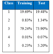
In the machine learning literature, it has been pointed out that little work has been done in the area of classification by machine learning when there is a highly skewed distribution of the class labels in the data set. In many cases, a classifier tends to be biased towards the majority class resulting in poor classification rates on minority classes. As we can see in the training and test class distribution of the KDD cup 1999 data U2R and R2L attacks constitute 0.24% of the training dataset but these attacks take up 5.27% in the test data.
Below is the class distribution table of KDD Cup 1999:
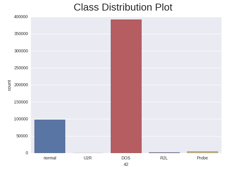
Below is the class distribution of the training set:
Below is the class distribution of the test set.
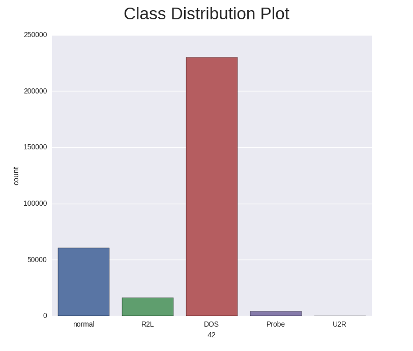
It is important to note that the test data is not from the same probability distribution as the training data, and it includes specific attack types not in the training data. This makes the task more realistic. Some intrusion experts believe that most novel attacks are variants of known attacks and the “signature” of known attacks can be sufficient to catch novel variants. The datasets contain a total of 24 training attack types, with an additional 14 types in the test data only.
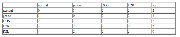
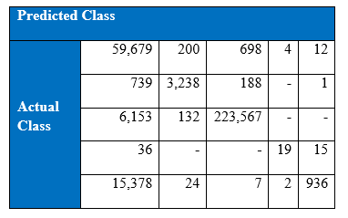
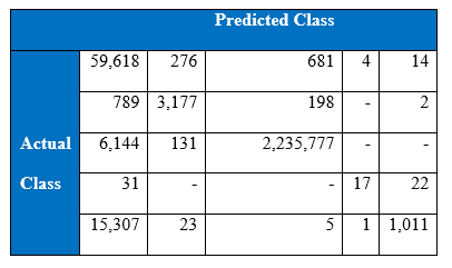
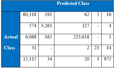
The winning entry of the KDD Cup 1999 is set as the benchmark for the project’s experimental results of KDD Cup 1999. The winning entry was submitted by Dr. Bernhard Pfahringer of the Austrian Research Institute for Artificial Intelligence using C5.0 decision tree classifier giving the benchmark for the comparison of our proposed machine learning algorithm. The winning entry achieved an average cost of 0.2331 per test example with the following confusion matrix:
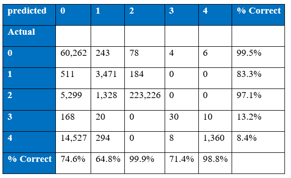
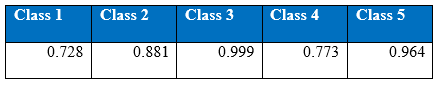
The last row represents the recall rate and the last column represents the precision. The main issue is that the recall rate of 8.4% for the last class by the winning entry is quite low. The winning entry’s classification technique is C5.0 Decision trees, a mixture of boosting and bagging, taking into account the minimization of the so-called conditional risk which is a similar approach as cost-sensitivity (introduced later). Bagging decision trees are random forests that represent an ensemble of decision trees averaged while training on different parts of the training set by sampling with replacement. Boosting is an iterative procedure used to adaptively vary the training set’s distribution in order for the base classifiers to focus on examples that are hard to classify. In boosting, weights are assigned to the data in such a way that examples that are misclassified gain weight and examples that are classified correctly lose weight. Below is the cost matrix that will indicate of the cost of misclassifying between the various class labels.
There are number of ways to evaluate the performance of a classifier:
Recall is the fraction of relevant instances that are classified.
Precision is the fraction of classified instances that are relevant.
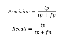
where tp : true positive which is the number of classes correctly predicted as belonging to the positive class
fp: false positive which is the number of classes incorrectly predicted as belonging to the positive class
fn : false negative which is the number of classes which were not predicted as belonging to the positive class but should have been.
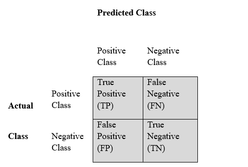
Confusion matrix also known as contingency table, is a table with rows and columns that reports the true positive, false positives, false negatives and true negatives as depicted in the figure below.
 F-1 score is the weighted average of the precision and recall that lies between 0 and 1. If the equal weighting is given to the precision and recall then the following formula is used;
![]()
where β corresponds to the relative importance of precision over recall. Instead of F1-score the average cost per test example is considered as an evaluation metric for the overall performance of the various learning algorithm techniques throughout this report.
When it comes to evaluating the performance of the classifier, it is better to rely on the precision, recall rates and F1-scores rather than accuracy levels. Let’s say we have a data set with a (0.9, 0.1) class distribution, there is the possibility that a classifier predicts everything as a major class and ignores the minor class. In that case, we get an accuracy level of 90% turning out to be a poor indicator of the performance of the classifier. There are better measures of performance of the techniques like the confusion matrix, recall (sensitivity), precision and F1-score.
Python is the primary programming language used in this project. Python has a lot of libraries that can be used for data manipulation and analysis. Scikit-learn is the most popular machine learning Python library that offers a variety of algorithms along with utilities for calculating confusion matrices, accuracy levels, recall and precision tables to evaluate the performance of a learning algorithm. A Python dictionary function was used to store the results of the network and the Python pickle function was used to retrieve stored results.
Python libraries like NumPy and Pandas were used extensively for data manipulation. A NumPy random seed is used to make sure that for every run the results are reproducible. Since the weights and biases are initialised randomly following a normal distribution, NumPy random seed is used so that the weights and biases initialised are the same in every run. Finally, the Matplotlib library was used for plotting. String formatting has been used to get separate graphs for different sets of parameters in the network.
Theano is the Deep Learning Python library that has been used in this project. Introduced as a CPU and GPU compiler by Bergstra at the Lisa lab of the University of Montreal in 2010, it allows defining, optimizing, and evaluating mathematical expressions involving multi-dimensional arrays efficiently. Below are some of the appealing features of Theano:
Import theano.tensor as T
Import numpy as np
T.dot(x,W_x) and np.dot(x,W_x)
Both implement the same function, the difference between the two is that NumPy uses numeric variables while Theano uses symbolic variables.
Theano is used for symbolic mathematical expressions that are compiled to a function that can operate on numerical data. For example,
x = T.vector("x")
y = T.vector("y")
fn = x*y
p = theano.function(inputs=[x, y], outputs=fn)
We can assign variables x and y using NumPy arrays to the numerical data of these variables which can then be used by compiled function like ρ above. To update a variable used in an equation (for example, while learning), Theano needs it to be in a special wrapper called a shared variable. Below are the model parameters for the first hidden layer in feedforward neural networks.
W_x = theano.shared(W_x, name="W_x")
b_h = theano.shared(b_h, name="b_h")
[global]
device=gpu
floatX=float32
Operations on data of type float32 are accelerated along with matrix multiplication and large element-wise operations especially when the arguments are large enough. The use of GPUs gives around 40x speedup over the use of CPUs particularly in larger networks. This feature of GPUs is one of the reasons for the revival and success of Deep Learning in the twenty-first century.
Theano has a large community that has been very helpful in developing the codes and assisting in their use. Error messages produced by Theano are quite different from the error produced by the standard Python packages because Theano codes are compiled. Therefore at times it had been difficult to understand the error message and debug the error.
In order to confirm that if our implementation of dropout is correct we decided to verify it on the well-known MNIST handwritten image dataset.
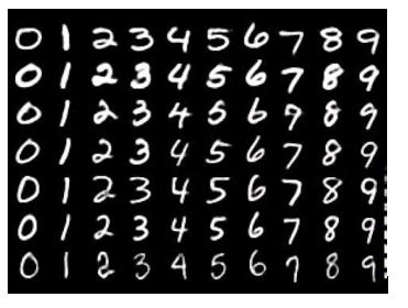
The famous MNIST handwritten digits image containing dataset digits 0 to 9 has been used for the experiments with 50,000 training examples, 10,000 validation examples and 10,000 testing examples. An image is represented as a 1-dimensional array of 784 (28 x 28) float values between 0 and 1 (0 for black and 1 for white). There is no need for pre-processing and formatting the data. MNIST dataset is one of the most well studied datasets in the area of computer vision and machine learning. It is based on two data sets collected by NIST, the United States’ National Institute of Standards and Technology. The NIST data sets were stripped down and put into a more convenient format by Yann LeCun, Corinna Cortes, and Christopher J. C. Burges.
An initial experiment was conducted to see the effect of dropout with a learning rate of 0.1 and no momentum. The figures below show the comparison.
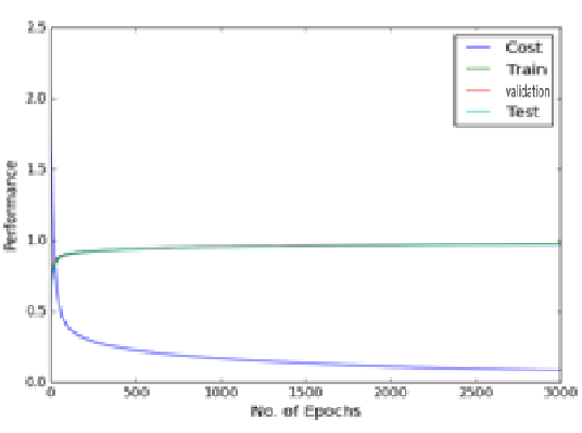
The experimental result of 2 hidden layers standard MLP of 800 hidden nodes with 3000 epochs
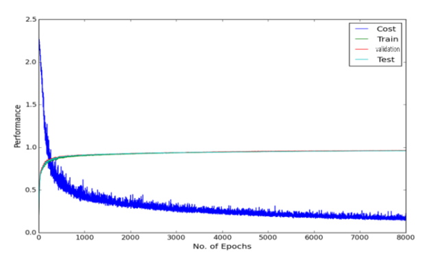
The experimental result of dropout on 2 hidden layers MLP of 800 hidden nodes and 8000 epochs as dropout made the learning of the network slower. Hence larger number of epochs is required.
As can be seen in the figure above there is a fluctuation in the training cost value (obtained by the cost function), and accuracies created by the dropout noise. Moreover it turns out that problem of local minima in the error surface is encountered in the dropout network (figure above depicts error surface with local minima). That is cost value plateaus at the higher value than at the value without using dropout, making the slow learning process for the network. Training cost value without using dropout is 0.083 while using dropout is 0.225 suggesting problem of local minima at the end of epoch of 3000 and 8000 respectively. Varying learning rate and momentum rate helps to solve the problem of local minima. It is little wonder that Hinton used various techniques to make dropout work.
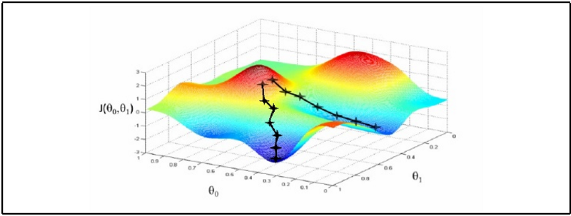
Depicts an error surface with poor local minima
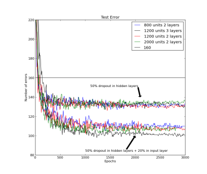
Hinton experiment results on MNIST
Hinton starts off his experiment with learning rate of 10 and exponentially decays the rate at 0.998 for each training epoch and then stabilizes the learning rate at 500 epochs. In order to prevent the model from blowing up, due to the very high learning rate, he puts an upper bound constraint on the squared length that is L2 norm of the incoming weight vector for each individual hidden unit. After cross-validation it turns out that maximum squared length of l = 15 give the best results. If a weight-update goes beyond the upper bound, weights are renormalized accordingly. Similarly he initially set the momentum rate at 0.5 and linearly increases to 0.99 over the first 500 epochs speeding up the training, in the subsequent epoch momentum rate stays constant at 0.99. We had to use 8000 epochs because learning is significantly slower with dropout. As per Hinton, adding dropout in the input layer with 20% random noise improves the result by quite a large margin. Apart from these hyper parameters, in the network architecture he uses stochastic gradient descent as an optimizer with mini-batches of 100 and a cross-entropy objective function.
In order to combat the problem of local minima we used some of the techniques of varying the learning rate and momentum over the epochs. The experiment started off at a learning rate of 0.1 and momentum of 0.2. The learning rate increased stepwise at 500, 1500, 3000 epochs decreasing to 0.08, 0.06 and 0.04 respectively at the same time momentum rate increased to 0.4, 0.6 and 0.8 at the same time. The testing accuracy level increased to 96.65% by varying learning rate and momentum as mentioned. The figurebelow shows the performance of the described networks.
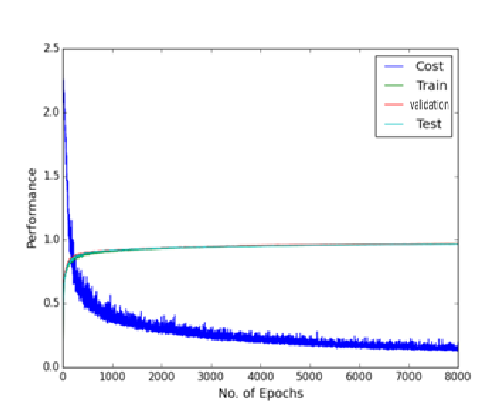
Table below is the comparison of our three experiments on the MNIST dataset. In the table test accuracy levels of three experiments can be seen. The number of epochs required to get the training costs were different for all three experiments.
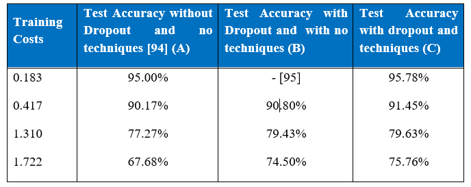
It can be seen that at various training cost levels experiment B result is better than experiment A’s. It took a network without dropout only 10 epochs to reach training cost of 1.310, whereas around 110 epochs were required to get the same training costs and thus better accuracy level by a network with dropout. Interestingly if learning rate and momentum are varied as in experiment C, not only accuracy level increases but also it takes fewer epochs, around 95 epochs, boosting the overall performance.
Later, we did the same experiment with 100-sized mini-batches along with the same architectures and parameters as before. It turns out that the mini-batches made the learning easier as it started off (in the initial epochs) with the higher training and testing accuracy levels and learning also converged quicker and at the higher level with testing accuracy level of 98.6%, getting closer to the benchmark.
It is very important to get data ready before doing any analysis. The treatment of categorical and continuous variables is quite different. Categorical variables are converted by one-hot encoding. In this encoding, a feature is obtained for each categorical variable in which one neuron/input represents each category, for example the following is the subset of two features in KDD Cup 1999 data set.
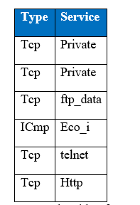
Sample with 2 features of KDD 99
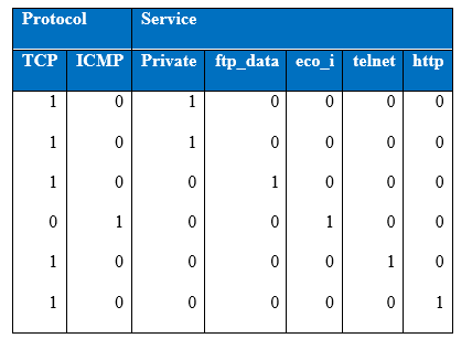
Table showing one-hot encoding of categorical samples
The first column of figure gives the binary representation of (tcp / not tcp) encoded as (0, 1) respectively, where tcp is represented in the above diagram as 1 and whichever example is not tcp is represented as 0. Similarly, the second column of figure above gives the representation of (icmp / not icmp). When all the variables are encoded from the first column of the categorical feature, the feature variables from the second feature type will be encoded in the same manner. As a result of one-hot encoding the input size has expanded from 42 units to 120 units.
Continuous features (attributes) have been transformed using the following rescaling;
 , where x is the value of the feature
One reason for scaling the data is to ensure that all variables are seen as equally important by smoothing out feature to feature variations. For example if feature A ranges between 1 and 100 while feature B ranges between 0.1 and 0.001, the network will assign smaller weights to feature A and larger weights to feature B. By rescaling all the features are brought to the same scale. Neural networks learn faster and give better result with pre-processed input variables as a result. All the samples in the dataset have been shuffled to ensure that if mini-batches are used then the training examples in the mini-batch will not necessarily have the same order of training sets in each mini-batch. Data shuffling randomizes the order of the data. However, instead of mini-batch training full gradient descent was carried out throughout this project.
In the raw data there was various attack types that were categorize into four main attack classes by following to compare with the winning entry’s method.
One of the challenging tasks in neural networks is to find the optimal hyper-parameters to get the best performance. It is always difficult to tell which combination of parameters works well. In the end these are all still heuristics most of the time. In the neural networks the parameter space is huge and it is difficult to explore each hyper parameter extensively. The experiments started with one hidden layer along with the hyper-parameter tuning. Hidden layers were then stacked and evaluated. Four hidden layers were the maximum that we have stacked and reported the results of. Moreover some techniques mentioned in the literature review were incorporated in to the learning algorithm like SMOTE, dropout and cost-sensitive learning. The experiments were conducted in full batch mode of back-propagation learning that is weights updated after all training examples were presented to the learning algorithm in each epoch. The cost is computed and parameters are updated to minimize the cost value. At the time of prediction of unseen examples the final updated parameters are used and there are no parameter updates.
Weights and bias are initialised using Python NumPy arrays. Weights are initialised using random standard normal distribution with mean zero and standard deviation of 0.05. Biases are initialised with values of zero.
One hidden layer MLP implementation in Theano was taken from one of the study and from there we worked all the way and changed the code to incorporate various other techniques. In the implementation one more hidden layer is stacked by initialising weights and biases the same way as in one hidden layer MLP. Same goes on for three and four hidden layer MLPs given in the subsequent sections of the report.
Theano codes for momentum, dropout and rectified linear units were fetched from the online Theano user community. The value of the momentum has to be multiplied by the parameter update of previous epoch to get the value of parameter updates of current epoch. To implement rectified linear units Theano’s maximum function was used so that the value of the hidden layer stays non-negative resulting in the sparsity. Theano already had a module for tangent activation functions. In the implementation of dropout, Theano Bernoulli function is multiplied by each hidden layer function in order to drop the weights and biases with probability p at the time of training. For the test using unseen data separate hidden layers are written with the same value of initialised / updated weights and biases being used but this time weights are scaled down by probability of .
SMOTE has been implemented by using Costcla Python library which is built on top of Scikit- learn, Pandas and NumPy. Cost-sensitive learning classification has been implemented in detailed in the further article.
The vanishing gradient problem was solved by using Rectified Linear Units as activation functions as these introduce sparsity effect on the networks. In order to evaluate the results, confusion matrix, recall rate, precision and cost per test sample have been considered because of the class imbalance problem. Accuracy levels of training and testing set have also been calculated to see when the network actually over-fits. Cross-validation does not seem to be an appropriate way to evaluate the performance and get the optimal results. It is because the distribution of the training set and test set is quite different. Cross-validation uses one subset of training data for learning and another subset of training data is used for validating. We used the subset of the training set for learning and the remaining subset of the training set for validating. It turned out that accuracy level of the validation set (subset of training data) was very high (higher than the accuracy level of the test set) confirming that the distribution of training and test set is quite different making the problem challenging.
All the experiments were done on CPU (not GPU). Some of the experiments took days to finish. As the network was grown bigger, computation became time consuming task. The four hidden layer MLP network with dropout was the largest network experimented in this project and it took around four days to finish that experiment with no hyper-parameter tuning which is described in section 4.3.5. Tuning hyper-parameters of the networks was the most time consuming part of the exercise. Three and four hidden layers MLP usually took a day to finish running with each set of hyper-parameters.
Initially a single hidden layer MLP was used in the experiments to get the optimal configurations and architecture. Description of the hyper-parameter search is given as follows.
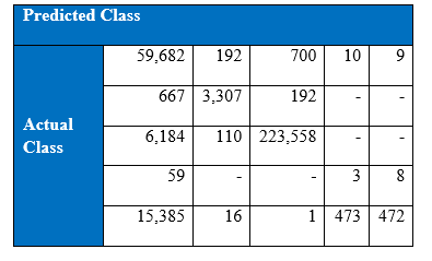
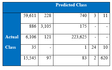
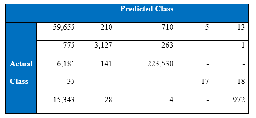
At the time of hyper-parameter tuning, a learning rate of 0.8 was chosen among the arbitrary set of 0.01, 0.1, 0.5, 0.8, 0.9, 1.0 and 1.2. Momentum of 0.8 was also chosen after hyper-parameter search. It is surprising to see a large learning rate along with large momentum to work well together because it is general practice to use a lower learning rate along with a large momentum to ensure that training cost oscillates smoothly down in the error surface while learning. However, since we are using full batch gradient descent a higher learning rate seems reasonable. Using an activation function of rectified linear units turns out to be better than the tangent units. Cost function of Negative Log-Likelihood (NLL) is chosen because of the softmax function in the output layer. It does not mean that NLL is the only cost function that can be used when softmax is in the output layer. Cost per test sample turns out to be 0.2472 by the standard single hidden layer MLP after hyper-parameter tuning. Cost per test sample is calculated by multiplying the confusion matrix given below and cost matrix given in section 1.3.3 and then divided by the total number of test examples which is around 0.3 million. Below are the graphical and tabular results of the network.
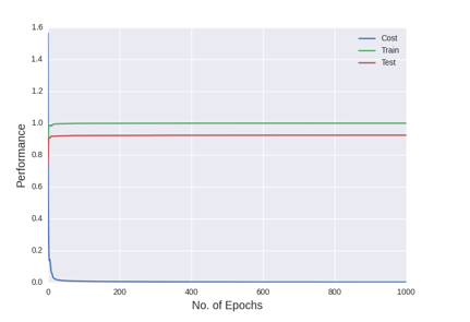
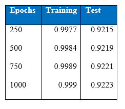
Figure shows the cost, and training and test accuracies levels of single hidden layer MLP after all the hyper-parameter selections
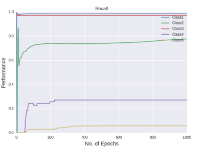
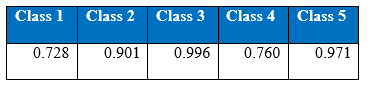
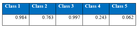
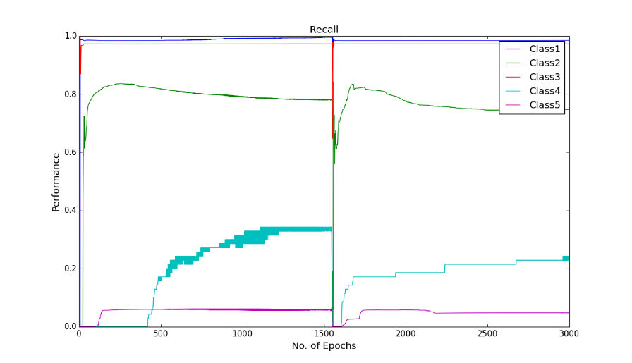
Figure shows the recall curves of all the five classes after all the hyper-parameter selections
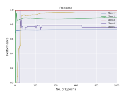
Figure shows the precision curves of all the five classes after all the hyper-parameter selections
Confusion Matrix by the last 1000 epoch:
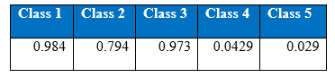
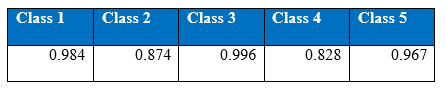
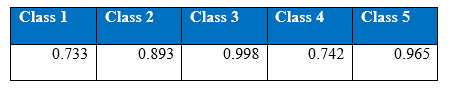
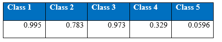
Recall by the last 1000 epoch:
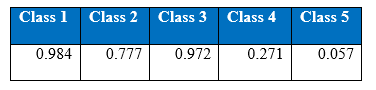
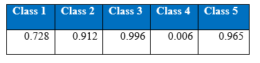
Precision by the last 1000 epoch:
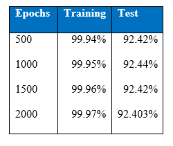
 In figure above, we can see that there is a gap between the training and test accuracy. This gap has been observed in all the experiments of the project. Training accuracy has been around 99% and test accuracy has been around 92%. This gap is due to the different distribution of training and test datasets. When portion of the training set was taken as the validation set, that same gap was not observed.
The figures gives out the recall and precision results respectively. As we can see the performance of the minority class of 4 and 5 is quite low. Hence we tried several approaches to deal with the class imbalance problem. After getting the results of one hidden layer of MLP, the objective of this project is to get the better results.
SMOTE-MLP for KDD Cup 1999 data
SMOTE is a technique to oversample the minority class by creating synthetic examples of minority class. SMOTE was used to increase the samples of minority class of U2R and Probe to 0.83% which is the proportion of R2L attack type from the proportion of 0.01% and 0.23% respectively. After the pre-processing step of oversampling the minority class along with data pre-processing step described in section 3.3 the processed KDD Cup 1999 data is tested on the single hidden layer MLP with the same architecture that is after hyper-parameter tuning.
The overall performance of the network on the data pre-processed by SMOTE has declined as can be seen in figure precision and figure recall. The lower performance of the network can be explained by the fact that the synthetic examples created by SMOTE makes them very similar to the majority attacks in the feature space. As a result the network is confusing between the minority class with the synthetic examples and the majority classes.
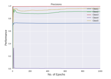
Figure shows the precision curves of all the classes by the one hidden layer MLP with SMOTE
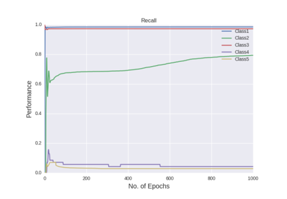
Figure shows the recall curves of all the classes by the one hidden layer MLP with SMOTE.
Recall at the end of 1000th epoch:
Precision at the end of 1000th epoch:
 Confusion matrix at the end of 1000th epoch
 It can be seen from the above tabular results, the performance of the minority classes has decreased. One possible way to improve the results is to try tuning the parameter. If we refer to previous section on SMOTE, the difference between the data generated by K-nearest neighbour and the original point is multiplied by a random number in the range 0 to 1. It will be interesting to see if we vary the range of this random number. Let’s say that this random number instead belong in the range of 0 to 0.5. If the minority classes with the synthetic samples stay indistinguishable from the majority attack classes, there might be an improvement.
There are three methods for the cost-sensitive learning of neural networks. The first method, cost-sensitive classification, was implemented into the single hidden layer MLP with the same architecture that is after hyper-parameter tuning. The cost matrix is given in section 1.3.3 where the cost of misclassifying the R2L as normal is 4 and similarly, the cost of misclassifying the normal as R2L is 2. P(i) is an estimate of the prior probability that an example belongs to the i-th class. The following table is the proportion of the training data set considered as P(i) in the computation.
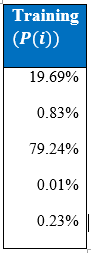
While testing there is a function in the implementation Theano code that selects the class index with the highest index value and sets that class index value to 1 and assigns 0 to the rest of the class. Therefore, there is no need to normalize P'(i) with denominator of ![]() .The cost vector represents the expected cost of misclassifying an example that belongs to the ith class.
.The cost vector represents the expected cost of misclassifying an example that belongs to the ith class.
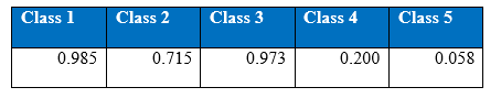
 Recall at the end of 1000th epoch:
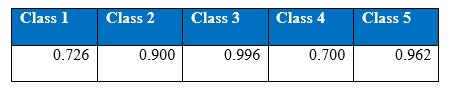 Precision at the end of 1000th epoch
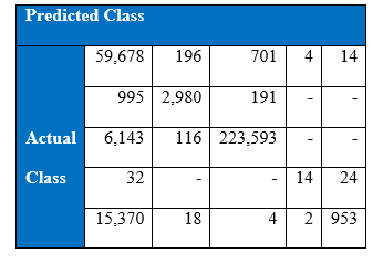
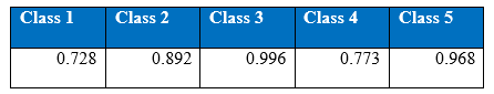
 As a result of cost-sensitive learning in the neural networks the correct classification of minority class 5 has increased from 936 to 953 increasing the recall rate to 5.83% at the 1000th epoch. This shows that given the appropriate misclassification cost table, our learning algorithm can adjust so that expected cost of misclassification for various classes goes down.
Below is the table of the comparison of test accuracy of one hidden layer MLP and one hidden layer MLP with cost-sensitive learning. As can be seen there is an overfitting by MLP with cost-sensitive learning where test accuracy declines after 750 epochs while training accuracy improves because it is supposed to stay intact in the cost-sensitive learning procedure. On the other hand, one hidden layer MLP’s test accuracy remains the same. Trade-off for cost-sensitive classification is that since the modified network is biased towards classifying the minority class that carries higher misclassification costs, the classification performance for the majority class may go down as it is can be seen in the below table.
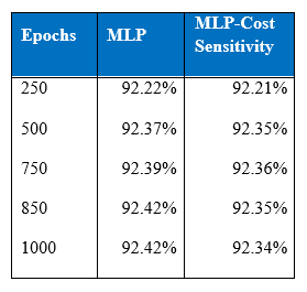
One of the popular ways neural network models deal with over-fitting is to use an early stopping rule. Training of cost-sensitive learning neural network can be halted after around 750 epochs which is when model starts to over-fit.
As more hidden layers are stacked it became apparent that the distribution of the number of hidden nodes needs to be changed as well. If more hidden layers are added then it is not necessary to have 175 hidden nodes in the first hidden layer. There is a distributed representation of the feature learning by the hidden nodes in the multiple hidden layers of the neural networks. Same configuration has been used as for the one hidden layer MLP apart from the hidden nodes. After hyper-parameter search from the following set of hidden nodes (175, 85), (175, 175), (100, 75), (75, 75), (75, 50), (100, 50), (75, 100), (100, 100) and (175, 150)
175 and 150 hidden nodes have been chosen for first and second hidden layers respectively for two hidden layers MLP. Single hidden layer MLP with 175 hidden nodes gives a better result than two hidden layer MLP. Cost per test sample is 0.2507. Below is the confusion matrix, precision and recall of the test set:
Precision at 1000th epoch:
Recall at 1000th epoch:
 There seems to be no improvement in the performance of the two hidden layer MLP. Below is the performance of accuracy level over the 1000 epochs:
Set of (100, 50, 75) were chosen for nodes of three hidden layers from the sets (100,50,35), (100,50,75), (100,75,35), (100,75,75), (175,150,50),(175,100,50) after hyper-parameter tuning. Architecture is same as multilayer perceptron with one or two hidden layers. It would have been interesting to see the effect of changing the remaining parameters like learning rate, momentum, etc on deeper network experimental results. However due to time-constraints it was not possible to carry that out.
Interestingly this network performed quite well on the class 4 (minority). And cost per test data sample is 0.2466 which is better than the single hidden layer MLP. Below is the confusion matrix, precision recall and accuracy tables;
Precision at the end 2000th epoch:
Recall at the end of 2000th epoch:
It can be seen that the precision and recall for minority class have improved. Number of epochs varies with the number of hidden layers. This is because it takes more time for the network to detect the minority classes and for the training cost to converge. Interestingly, training accuracy improves quicker as more hidden layers are stacked.
One of the objectives of this article is to see the performance of dropout. In this experiment higher number of nodes is tested with the intention to use dropout (later with the same setup) to regularize and avoid over-fitting in the network. This was done deliberately to ensure that the network is expressive enough to benefit from the dropout. In Hinton said that if the network does not over-fit, make it bigger. In the three hidden layers MLP there seemed to be insignificant overfitting over 2000 epochs. Applying Hinton’s advice, one more hidden layer was stacked and this time added more hidden nodes across the hidden layers. Number of hidden nodes that is used was as follows 375, 200, 150, 75 for first, second, third and fourth hidden layers respectively. Table below is the performance of four hidden layers MLP.
Cost per test sample is 0.2466. It seems like as more hidden layers are stacked the cost per test sample seems to go down. Over-fitting is seen after 1500 epochs as test accuracy goes down while training accuracy stays around the same.
Confusion matrix at the end of 3000th epoch:
Precision at the end of 3000th epoch
Recall at the end of 3000th epoch:
 Interestingly both training and test accuracy levels of four hidden layers MLP are higher than single hidden layer MLP’s. The performance of the minority classes has also improved as depicted by above tables. Now cost-sensitive learning classification will be integrated to boost the performance of the minority classes.
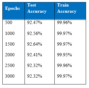
Cost-sensitive classification method was used here as well. This technique is incorporated into four hidden layer MLP. Table below is the performance of four hidden layers MLP with cost sensitive classification:
Cost per test sample is 0.2424 and test accuracy of 92.64% was achieved at the end of 1500 epoch. These values have been the best that had been achieved throughout this project.
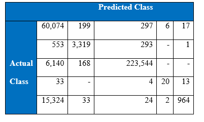
Confusion matrix at the 1500th epoch:
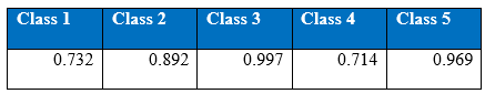
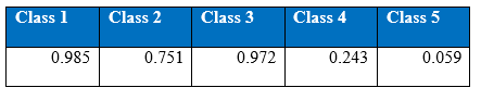
Precision at the 1500th epoch:
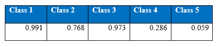
Recall at the 1500th epoch:
 It is interesting that the neural networks for the class imbalance problem improves when more hidden layers are stacked, that is, if we build deeper networks, the performance on the minority classes gets better than with a shallower network. Throughout the iteration, the maximum correct number of classifications of minority class 5 has been 964, boosted to around 1000 correct when cost-sensitivity in the classification was incorporated. The performance of the minority class worsens after 1300 epoch, and after 1500 epochs the performance of the overall test accuracy starts to decline. Below is the graph of the recall for the classes.
Dropout used in cost-sensitive learning in four hidden layer MLP for KDD Cup 1999 data
Finally, dropout regularisation is used with a cost-sensitive learning four hidden layer MLP to combat the over-fitting and investigate if the network performs. 2.5% of the noise level was added into the network by dropout. 2.5% is chosen because the use of dropout regularisation makes the learning a lot slower and we varied learning rate and momentum. In the beginning of this experiment, learning rate of 0.8 and momentum of 0.2 was used. Then learning rate changed to 0.6, 0.2 and 0.05 stepwise, momentum changed to 0.4, 0.8 and 0.85 stepwise at the epoch of 500, 1000 and 1500 respectively. Below are the performance graphs of the network. Spikes and fluctuations are seen in the training cost curve, precision and recall curves particularly for the minority classes in figures. This gives less confidence to use dropout in the network to make predictions.
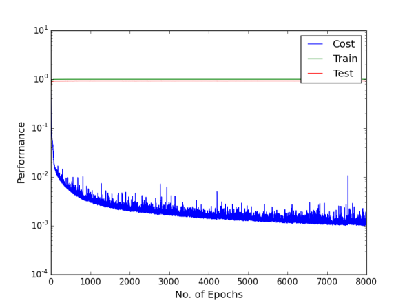
Figure shows the cost, and training and test accuracies levels using Deep MLP network with dropout of 2.5%
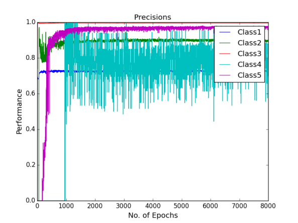
Figure shows the precision curves of all the classes using Deep MLP network with dropout of 2.5%
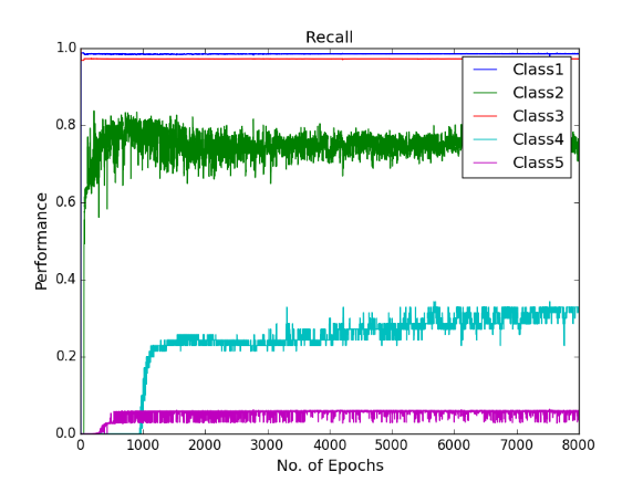
Figure shows the recall curves of all the classes using Deep MLP network with dropout of 2.5%
Cost per test sample is 0.2477; it is calculated by the multiplying confusion matrix given below with cost matrix. Below are the confusion matrix, recall and precision tables;
Precision
Recall
 There are other regularisers used in neural networks like weight decay L2 that deals with the overf-fitting. It will be interesting to see the comparison of dropout with other regularisers. Using dropout does not seem to give any advantage.
This article addresses the problem of anomaly detection through proper classification. SMOTE, sampling approach to deal with the class imbalance problem can do well if features of the different classes are distinguishable. It will be interesting to see the performance of the data resampling by SMOTE on the binary classification to distinguish between the normal and intrusion connections in the KDD cup 1999 data.
Cost-sensitive learning of neural networks seems to be effective in dealing with the class imbalance. The overall accuracy of 92.64% turns out to be the best result achieved by us by cost-sensitive classification of deep four hidden layer neural network. In another research by Kukar et al, Adaptive learning rate and minimization of the misclassification costs were concluded to be more effective than the cost-sensitive classification (the method that is actually implemented in this project is cost-sensitive classification). It will be interesting to see the performance of the network with those two other cost-sensitive learning methods of adaptive learning rate and minimization of the misclassification costs.
Not only can cost-sensitive learning be adopted in network intrusion and classification problem but also in various other areas like in healthcare applications. For example the cost of misclassifying if a person is not likely to have a disease when they actually are likely to have one is more than the cost of misclassifying a person who is likely to have a disease but actually does not. We have applied cost sensitive learning here (like they do in healthcare) because here, like healthcare too, the cost of a false negative or misclassification can be huge for false positives and spark mass litigations in cyber breaches. Having to deal with a bit more false positives makes it worth it to have lower false negatives.
Cost-sensitive learning seemingly has worked quite well in most of the research projects when dealing with the class imbalance problem. In the research by Dalyac the cost function called Bayesian cross entropy is introduced which tackles the problem of the image dataset using deep convolutional neural network. Bayesian cross entropy is simple modification of the equation of the cross entropy. In the Bayesian cross entropy, instead of assigning identical probability distribution to all the classes while trying to maximize the joint probability of occurrence, higher probability distribution to the minority class is assigned. This idea is very similar to the cost-sensitive learning. Below is the Bayesian cross entropy equation:
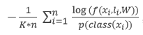 , where is the number of classes.
It turned out implementing any non-standard technique requires lot of work. If we had relied on a Deep Learning library like Pylearn2, the advantage would have been that we could have explored more techniques like Maxout, weight decay, etc. without worrying so much about the implementation, but the disadvantage would have been that we would not have had understood the implementation of techniques like Dropout extensively and may not have been able to implement highly customised changes.
While Deep Learning has shown remarkable success in the area of unstructured data like image classification, text analysis and speech recognition, there is very little literature on Deep Learning performed on structured/relational data which makes this investigation intriguing. After the extensive investigation carried out in this project, it does seem that Deep Learning has the potential to do well in the area of structured data. In Deep Belief Networks have performed well (better than support vector machine and single hidden layer MLP) on the KDD Cup 1999 data with class imbalance. In this project it has been observed that if more hidden layers are stacked the performance on the minority class improves to some extent.
Theano is particularly challenging as it is difficult to debug errors since Theano uses compiled functions. It would have been nicer, cleaner and avoided a lot of repetitive code if we had implemented the code in Python as an Object Oriented Programming (OOP) language. OOP can scale quite nicely as the program complexity grows. This is the approach of Pylearn2, Keras and other Deep Learning libraries.
Aside from pylearn2, tensor flow and H20 are also good alternatives. H20 can be used for Deep Learning in both Python and R. H20 has scalable, fast Deep Learning using mostly on the feedforward architecture. When using momentum updates for momentum training, H20 recommends using the Nesterov accelerated gradient method, which uses the nesterov accelerated gradient parameter.
It seems that if we are dealing with class imbalance problems then it is best to focus on the techniques that are specifically dealing with the class imbalance problem. On the other hand, Deep Learning shows the potential to optimise the results by that technique of stacking more hidden layers on the neural network.
Hinton has explicitly stated that dropout improves the performance of neural networks on supervised learning tasks in vision, speech recognition, document classification and computational biology. All these tasks have unstructured data. This questions if dropout actually works on the structured data like KDD 1999 Cup. Further experiments on structured data are required to solidify this tentative doubt.
An alternative to our method of using Multi-layer Perceptron can be utilizing Encoder-Decoder networks for structured data instead. Encoder-Decoder is a framework that aims to map highly structured input to highly structured output. This framework has been applied recently in machine translation where one language is translated by machine to another.
An alternative for handling class imbalance problem is using Deep Coding networks as they change parameters as context of data changes on another dataset (preferably not KDD 1999). This is very important for fraud and intrusion as fraudsters are continuously scheming new contexts and ways to deceive.
This project has shown that Deep Learning can be a powerful classification technique using categorical and continuous valued of the type typically collected by business processes. The expressive power of even relatively small neural networks has been seen in their ability to closely fit the large volume of training data. Deep Learning is clearly a powerful technique, and businesses may find many applications for it. However, it has also become clear through this project that considerable experience is required to get good results from Deep Learning. There are many architectures, techniques, and hyper-parameters that need to be carefully chosen before a model performs well on unseen data.
Companies can gain much from applying Deep Learning techniques in many areas, such as proper classification and other methods mentioned in the previous sections. Many techniques are still recent and until the foundations of Deep Learning are better understood, or more general deep models are developed, businesses must be prepared to invest in gaining experience and a certain amount of trial and error should be carried out before usable results are obtained.
We hope this article was a great value add for you. Tell us in the comments below if you found this study helpful or not. If you have any questions whatsoever, we are happy to answer them. Just post your questions in comments sections.
For all the deep learning practinors, if you have worked on KDD dataset, share your experience with us and what approach you followed. Now time to explore more. Go start your search now.
Lorem ipsum dolor sit amet, consectetur adipiscing elit,


Excellent analysis! Thank you so much. The learning would be complete if the python code is also made available.
Superb article, but it will be good if you provide us the same Train and Test data along with the python codes
Awesome! Want to learn more if the github address can be shown. Thank you!